
Have you ever carried out some job with out actually serious about the method concerned? For instance, making espresso, tying your sneakers, or strolling by way of your neighborhood.
In some of these actions, you’ve got carried out these items so many instances that you’ve got mastered the method. You will be serious about one thing unrelated, but you carry out these actions all the identical. This phenomenon known as procedural reminiscence in psychology.
We have this sort of factor with machine studying fashions as properly, nevertheless it’s not as constructive as it’s with people. This is named overfitting in machine studying.
What is Overfitting?
In overfitting, a mannequin turns into so good at our coaching information that it has mastered each sample, together with noise. This makes the mannequin carry out properly with coaching information however poorly with check or validation information.
The illustration beneath depicts how an optimum mannequin suits into the information in comparison with overfitting.
In the graph, we now have our options on the x-axis. In datasets, options are information that can be utilized to foretell an end result. The output variable is the end result based mostly on these options. The blue dots signify the information factors the place the options decide output variables.
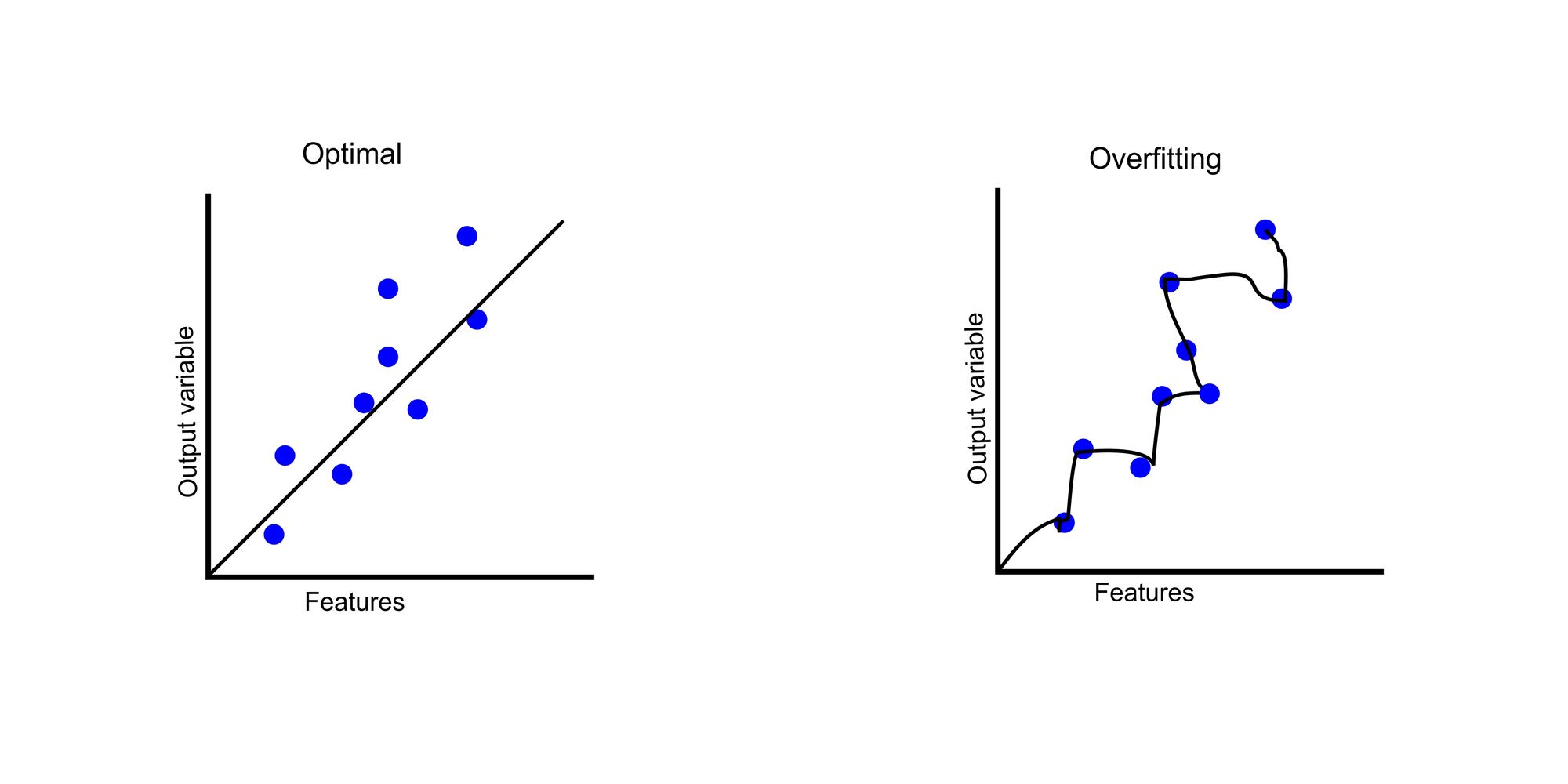
In the optimum graph, our mannequin tries to search out the generalized development. But in our overfitted chart, the mannequin tries to grasp every information level, leading to an asymmetrical curve.
An instance of a case examine can be to foretell if a buyer would default on a financial institution mortgage. Assuming we now have a dataset of 100,000 prospects containing options corresponding to demographics, earnings, mortgage quantity, credit score historical past, employment document, and default standing, we cut up our information into coaching and check information.
Our coaching dataset incorporates 80,000 prospects, whereas our check dataset incorporates 20,000 prospects. In the coaching the dataset, we observe that our mannequin has a 97% accuracy, however in prediction, we solely get 50% accuracy. This reveals that we now have an overfitting downside.
Can you inform why overfitting is an issue? Yes! It produces an incorrect prediction. It is the aim of machine studying fashions to make predictions to assist enterprise decision-making. We waste time and assets when our mannequin makes incorrect predictions.
Imagine predicting {that a} buyer pays again a mortgage, and the shopper defaults. Not only one buyer however hundreds of shoppers. This may cause a disaster for any monetary establishment.
Causes of Overfitting
Noisy information
Noise in information usually seems as errors, fluctuations, or outliers within the information. This will be brought on by information entry errors, information growing old, information transmission errors, and so forth.
Too a lot noise in information may cause the mannequin to assume these are legitimate information factors. Fitting the noise sample within the coaching dataset will trigger poor efficiency on the brand new dataset.
For instance, for example that we’re constructing a machine-learning mannequin to categorise pictures of cats and canines. But a few of the pictures within the dataset are blurry or poorly lit. While the mannequin could carry out properly on the coaching information, it would battle on the check information because it should have mastered some sample with the blurry pictures within the dataset.
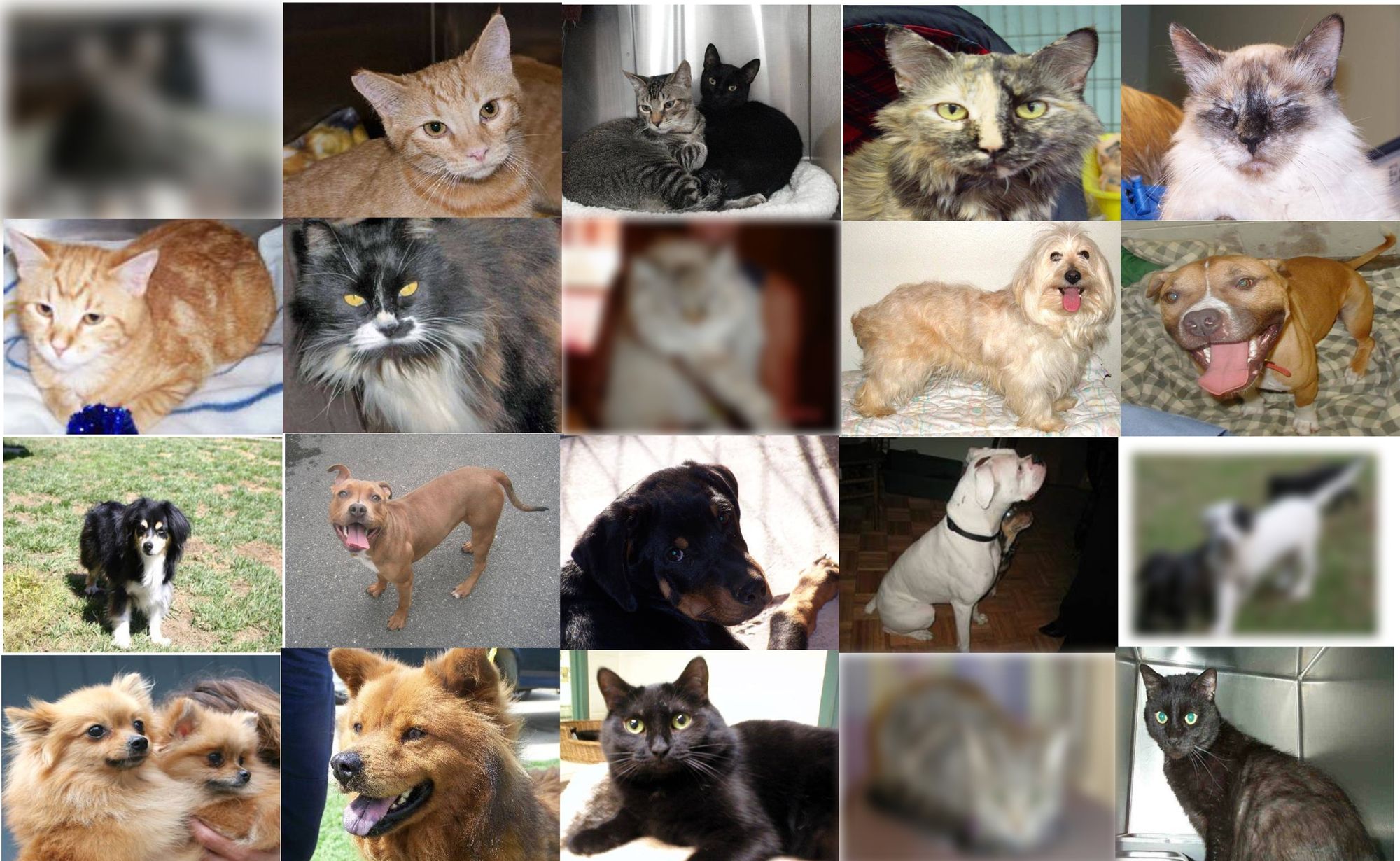
In the image above, you may see that we now have some blurry pictures that can’t be labelled if they’re cat or canine. In these situations, the mannequin may additionally study these patterns alongside related options. Removing these pictures can scale back overfitting.
Insufficient coaching information
There can be fewer patterns and noises to investigate if we do not have enough coaching information. This signifies that the machine can solely study a bit about our information.
Using our earlier instance, if our coaching information incorporates fewer pictures of canines however many extra of cats, the mannequin learns a lot about cats that once we feed the system a picture of a canine, it should probably give a improper output.
Overly advanced mannequin
In a posh mannequin, there are lots of parameters able to capturing patterns and relationships in coaching information. As a end result, our mannequin makes a extra correct prediction.
But this will pose an issue, because the mannequin can begin capturing noise, fluctuations, or outliers. Let’s have a look at a choice tree mannequin, the way it works, and the way overfitting can occur when it turns into too advanced.
A choice tree mannequin works by repeatedly breaking down information into vital options, making every level a node. This creates a tree like construction.
To make a prediction, it begins from the basis node and comply with the branches down, breaking and becoming each characteristic till it will get to the leaf node. The prediction is then made based mostly on the worth related to the leaf node.
Let’s have a look at a easy tree diagram of how a choice tree can predict if a buyer is more likely to default on mortgage base on sure options.
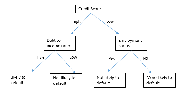
This mannequin begins by making a mother or father node which is credit score rating. Depending on whether or not the credit score rating for the applicant is excessive or low, it goes right down to the following node, which is both debt to earnings ratio or employment standing. Then it makes the ultimate prediction as as to whether the shopper is more likely to default or not.
A choice tree can turn out to be overly advanced when it creates too many nodes, making it too detailed or particular to the coaching information.
Let’s see a pattern machine studying program that predicts whether or not a buyer will default a mortgage or not utilizing choice tree mannequin. For specificity, I wont be exhibiting the cleansing course of and visualization. I’ll simply lay emphasis on the required capabilities and the way overfitting can occur with choice tree mannequin.
The hyperlink to the whole repository containing cleansing and visualization will be discovered right here, and you may get the dataset right here.
import pandas as pd
import numpy as np
import matplotlib.pyplot as plt
import seaborn as sns
from sklearn.metrics import accuracy_score
from sklearn.model_selection import train_test_split
from sklearn.preprocessing import LabelEncoder
from sklearn import tree
from sklearn import metrics
from sklearn.tree import ResolutionTreeClassifier

%matplotlib inline

#Importing our libraries
prepare = pd.read_csv('/content material/prepare.csv')
check = pd.read_csv('/content material/check.csv')

#Combine each coaching and check information
df = pd.concat([train, test], axis=0)
df.head()

#View dataset
prepare.head()

# Copy require options to a variable df_
df_ = prepare[['Gender',
'Married',
'Education',
'Self_Employed',
'Dependents',
'ApplicantIncome',
'CoapplicantIncome',
'LoanAmount',
'Loan_Amount_Term',
'Property_Area',
'Credit_History']]

### Duplicate a replica of df into X
X = df_.copy()

### label encode for Y
y = prepare['Loan_Status'].map({'N':0,'Y':1}).astype(int)

### train-test cut up
X_train, X_test, y_train, y_test = train_test_split(X, y, test_size=0.2, random_state=42)

# prepare
clf = ResolutionTreeClassifier() #change mannequin right here
clf.match(X_train, y_train)

# predict
predictions_clf = clf.predict(X_test)

#Print Accuracy
print('Model Accuracy:', accuracy_score(predictions_clf, y_test))
To perceive this higher, I’ll clarify what every module does:
import pandas as pd
import numpy as np
import matplotlib.pyplot as plt
import seaborn as sns
from sklearn.metrics import accuracy_score
from sklearn.model_selection import train_test_split
from sklearn.preprocessing import LabelEncoder
from sklearn import tree
from sklearn import metrics
from sklearn.tree import ResolutionTreeClassifier
The first block is the import part. This is the place we import all our dependencies.
- Numpy is a Python library used for scientific computing.
- Pandas is a library for information evaluation and manipulation.
- Matplotlib and Seaborn are for statistical information visualization.
Accuracy_scoreis a operate to calculate the accuracy of our mannequin.train_test_splitis used to separate our dataset into coaching and check information.- The
LabelEncoderencodes categorical variables into numeric variables. treeis for constructing a choice tree classifier.metricshelps us consider our fashions.
#Importing our dataset
prepare = pd.read_csv('/content material/prepare.csv')
check = pd.read_csv('/content material/check.csv')
This module imports our datasets. Our prepare and check datasets have been downloaded from the general public repository, so we import them individually.
#Combine each coaching and check information
df = pd.concat([train, test], axis=0)
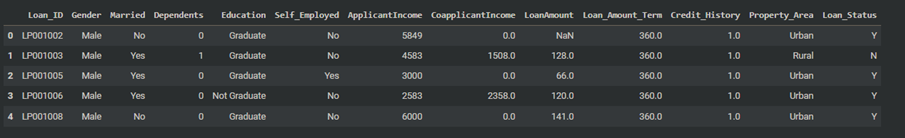
df.head()
To work with each datasets, we have to mix them into one dataset. The concat operate combines each datasets. We use df.head() to visualise the dataset which is proven beneath.
# Copy require options to a variable df_
df_ = prepare[['Gender',
'Married',
'Education',
'Self_Employed',
'Dependents',
'ApplicantIncome',
'CoapplicantIncome',
'LoanAmount',
'Loan_Amount_Term',
'Property_Area',
'Credit_History']]

### Duplicate a replica of df into X
X = df_.copy()
To begin working with our options, we created a variable df_ to retailer all of the options wanted for prediction. We duplicated this into the variable X to create a replica to work with.
### label encode for Y
y = prepare['Loan_Status'].map({'N':0,'Y':1}).astype(int)
To work with our end result variable, we would have liked to transform it from a categorical worth to an integer worth. This additionally makes it straightforward for our mannequin to know. All values of N have been transformed to 0, whereas Y was transformed to 1.
### train-test cut up
X_train, X_test, y_train, y_test = train_test_split(X, y, test_size=0.2, random_state=42)
We use our train_test_split to separate our information into coaching and check information. The test_size = 0.2 means we’re utilizing 20% of the information for testing and 80% for coaching.
# prepare
clf = ResolutionTreeClassifier()
clf.match(X_train, y_train)
We assigned ResolutionTreeClassifier() to the variable clf, which we’ll use to coach and match our information. ResolutionTreeClassifier() has an optionally available argument named max_depth. The quantity assigned to max_depth determines the depth of the tree. This is how we’ll use it to trigger overfitting in one other part beneath.
# predict
predictions_clf = clf.predict(X_test)
In the code snippet above, clf.predict is used to foretell the information in X_test.
print('Model Accuracy:', accuracy_score(predictions_clf, y_test))The mannequin accuracy was printed utilizing the accuracy_score operate, which you’ll see within the screenshot beneath:

Now that we have seen how a choice tree works and even run a machine studying mannequin to foretell if a buyer will default or not, let’s examine the right way to trigger and diagnose overfitting by modifying the code utilizing the max_depth argument.
How to Diagnose Overfitting
Visualizations
Using visualizations can assist us detect overfitting by offering insights into the conduct of our mannequin.
Common visualization strategies embrace plotting information factors for the mannequin’s prediction, visualizing characteristic distributions, or creating plots of choice boundaries.
To visualize the overfitting for our mortgage software above, I needed to tweak the code by creating an iteration utilizing totally different max_depth values starting from 1 to 24. Predictions are calculated based mostly on coaching and check information and saved in a listing.
#Creating a listing to retailer accuracy values
train_accuracies = []
test_accuracies = []

#Loop
for depth in vary(1, 25):
  tree_model = ResolutionTreeClassifier(max_depth = depth)
  tree_model.match(X_train, y_train)

  train_predictions = tree_model.predict(X_train)
  test_predictions = tree_model.predict(X_test)

  #calculate coaching and check accuracy
  train_accuracy = metrics.accuracy_score(y_train, train_predictions)

  test_accuracy = metrics.accuracy_score(y_test, test_predictions)

  #Append accuracies
  train_accuracies.append(train_accuracy)
  test_accuracies.append(test_accuracy)
The distinction right here is that we’re creating two variables – train_accuracies and test_accuracies – to retailer the accuracy values. Using these variables, we are able to use the code beneath to generate a plot that reveals the adjustments between these variables because the max_depth worth adjustments.
#Creating our plot
plt.determine(figsize = (10, 5))
sns.set_style("whitegrid")
plt.plot(train_accuracies, label= "prepare accuracy")
plt.plot(test_accuracies, label="check accuracy")
plt.legend(loc = "higher left")
plt.xticks(vary(0, 26, 5))
plt.xlabel("max_depth", measurement = 20)
plt.ylabel("accuracy", measurement = 20)
plt.present()
This is how the plot seems to be:
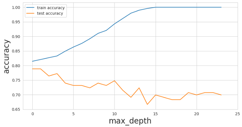
You’ll discover that as max_depth values on the x-axis start to extend, the coaching information accuracy begins enhancing loads to an ideal rating. In spite of this, the check information accuracy decreased from 0.78 to 0.70. This is a traditional instance of overfitting because the mannequin turns into too advanced.
Training and validation accuracy hole
The accuracy hole is an effective approach to know if overfitting has occurred in your program. This means that there’s a huge hole between coaching information and validation information in terms of accuracy.
As a information, a 5% hole is what you must search for. Cases the place you have got greater than this are sometimes an indicator of overfitting: for instance, our visualization above reveals that when our max_depth worth was at 2o, our coaching accuracy was at 100% whereas our check accuracy was 70%.
How to Prevent Overfitting
Collect extra coaching information
As mentioned above, inadequate coaching information may cause overfitting because the mannequin can not seize the related patterns and intricacies represented within the information.
Machine studying typically requires hundreds or hundreds of thousands of information in your dataset for coaching. With this, there can be sufficient patterns to seize. You can determine outliers or noise extra simply in case you’ve carried out correct cleansing on the dataset utilizing related methods.
Use regularization methods
Regularization methods contain simplifying fashions by penalizing much less influential options. These penalties are embedded within the mannequin’s loss operate.
Regularization methods for the choice tree mannequin above embrace pruning, value complexity pruning, and others.
Pruning is a method that entails eradicating pointless branches from the choice tree. For instance, we are able to set a minimal variety of prospects on a leaf, corresponding to 20. This prevents the tree from making selections based mostly on a really small group of shoppers.
Cost complexity entails eradicating branches from the tree based mostly on their complexity. This controls the trade-off between tree complexity and accuracy.
Ensembling
Ensembling entails combining a number of machine studying fashions to contribute their strengths and distinctive views to make a prediction.
Ensembling leverages the knowledge of the gang to make extra correct predictions on unseen information, which improves generalization and reduces the danger of overfitting.
Popular ensemble strategies embrace bagging, boosting, and stacking, which have been profitable in a variety of machine-learning duties.
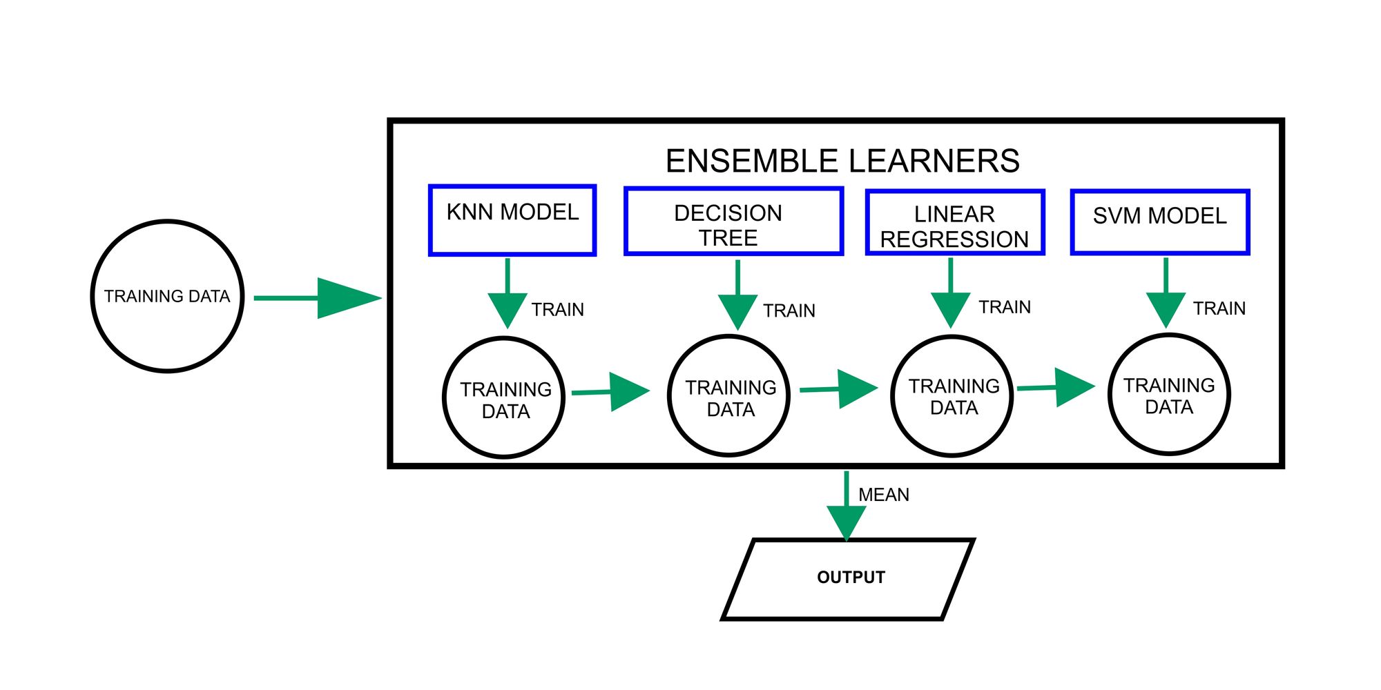
The diagram above reveals how the ensembling methodology combines numerous machine studying fashions for making predictions. Each mannequin is skilled independently on its respective subset of information. The predictions for particular person fashions are then mixed or the imply is gotten to make a remaining prediction.
Conclusion
Overfitting occurs when a mannequin suits coaching information too carefully, leading to nice coaching efficiency however poor generalization. Overfitting will be problematic because it yields incorrect predictions.
This will be brought on by an absence of coaching information, an excessively advanced mannequin, or noisy information. Diagnosis entails assessing the training-validation accuracy hole, utilizing visualizations to scrutinize mannequin conduct, and so forth.
Prevention methods embrace amassing extra coaching information, utilizing regularization methods, and using ensemble strategies. These approaches guarantee fashions generalize properly and make correct predictions for knowledgeable selections.
Thank you for studying! Please comply with me on LinkedIn the place I additionally put up extra information associated content material.