Large Medical Picture Preprocessing With Apache Beam

Utilizing synthetic intelligence in healthcare is fraught with challenges. 

A singular downside within the subject is heavy enter codecs. Tissue samples are sometimes digitalized in ultra-high decision. And the file measurement of those photographs will be a number of gigabytes, making them inconceivable to load in a generic picture viewer (on account of an absence of reminiscence to accommodate a deserialized picture). 

That’s why we should pay explicit consideration to preprocessing when utilizing significantly giant photographs with any synthetic intelligence mannequin. This text will stroll you thru find out how to course of giant medical photographs effectively utilizing Apache Beam — and we’ll use a particular instance to discover the next:

• Learn how to strategy utilizing big photographs in ML/AI
• Totally different libraries for coping with stated photographs
• Learn how to create environment friendly parallel processing pipelines

Prepared for some severe knowledge-sharing? 

Let’s get began!

Background: Mayo Clinic STRIP AI competitors

This text is predicated on our latest expertise on the Mayo Clinic STRIP AI competitors organized by Kaggle.

Kaggle is an internet neighborhood for information scientists that repeatedly organizes information science contests. In every contest, contributors get an issue and an related dataset earlier than being tasked with making a mannequin that greatest solves the difficulty at hand. 

The options are then ranked, and the highest rivals obtain a prize. Typically, the issues come from exterior entities making an attempt to make use of the neighborhood to search out proof of idea AI options to issues of their area. One such entity is The Mayo Clinic: a non-profit American educational medical middle centered on built-in healthcare, schooling, and analysis.

The Mayo Clinic sponsored the Mayo Clinic – STRIP AI competitors centered on picture classification of stroke blood clot origin. The purpose was to categorise the blood clot origins in an ischemic stroke. Utilizing whole-slide digital pathology photographs, contributors needed to construct a mannequin that differentiates between the 2 main acute ischemic stroke etiology subtypes: cardiac and enormous artery atherosclerosis.

The usual remedy for an acute ischemic stroke is mechanical thrombectomy (clot removing). After the occlusion is extracted from the affected person’s blood vessel, it’s doable to research the tissue pattern. The tissue is scanned in excessive decision and digitalized. A healthcare skilled (utilizing devoted viewer software program) can then use the scans to find out the stroke etiology and clot origin, which helps deal with the affected person and stop future strokes.

But it surely’s not simple to identify the tell-tale indicators in scans. That’s why the clinic needs to harness the ability of deep studying in a bid to assist healthcare professionals in an automatic means. Sadly, the competitors guidelines stop us from publishing competitors information publicly. 

So when you gained’t see precise samples, you’ll find a blood clot scan pattern under (taken from Orbit picture evaluation machine studying software program, used for the histological quantification of acute ischemic stroke blood clots).

A, C: Histopathological staining of an AIS clot with H&E stain, 1X & 10X respectively

Preprocessing challenges

Earlier than information scientists can apply deep studying to the tissue samples, the information must be preprocessed. Typical Neural Community architectures take comparatively small photographs (for instance, EfficientNetB0 224x224 pixels) as enter. This isn’t suitable with the picture sizes of the pictures within the unique dataset, which may attain tens of hundreds by tens of hundreds of pixels.

The preprocessing needed to extract significant information from the supply photographs whereas nonetheless being light-weight sufficient to run on Kaggle infrastructure inside a restricted time. We determined to implement the identical preprocessing pipeline for coaching and inference to make sure we didn’t introduce any skew.

The challenges that we confronted with preprocessing included the next:

• 395.36 GB of TIFF information as enter
• TIFF information that have been a number of GB in measurement
• Inference needed to run on restricted Kaggle cases (16GB RAM, 4 CPU, 20 GB persistent disk area)
• Inference needed to run inside a restricted submission time (9 hours for about 280 photographs)
• Preprocessing ought to be shared for coaching and inference (the coaching set had 754 photographs)

As a result of above elements, we have been compelled to make use of the machine’s CPU to the utmost whereas limiting reminiscence utilization. Apache Beam helped us parallelize our computations. libvips and openslide helped us take care of the large picture information.

The pipeline

Dataset construction

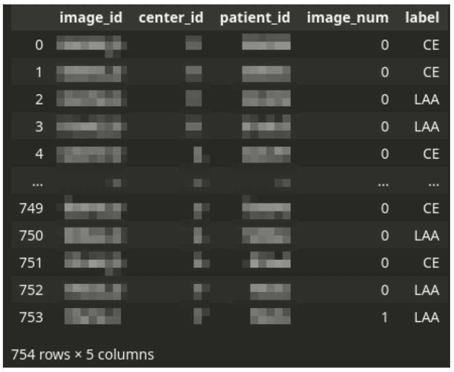
Censored coaching CSV file construction

The principle CSV file drives the dataset. The CSV file comprises one row for every tissue picture scan. Every affected person can have one or just a few photographs.

There’s all the time a single analysis, even from a number of photographs – the stroke subtype is assigned to a affected person, not a picture. Thus the dataset must be logically grouped by affected person ID.

The CSV file is accompanied by a set of giant TIFF photographs. Every picture corresponds to a single row within the CSV file. The TIFF information comprise digital scans of tissue slices. A single picture can have a number of fragments of tissue. There’s often a big space of the background. The background will not be all the time a strong shade – generally, there is perhaps a sample of a special shade.

The pictures comprise giant ineffective background areas which can be a primary goal for dimensionality discount – we are going to wish to discard the background areas from additional processing as they carry no useful data.

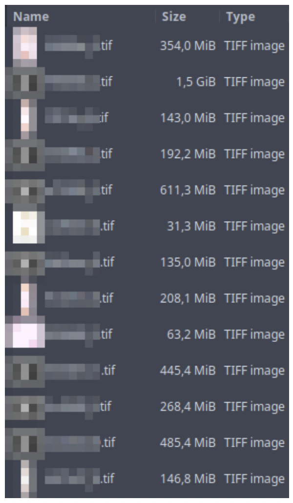
Censored fragment of photographs listing itemizing

A number of Occasion Studying

One affected person can have a number of photographs however a single analysis within the dataset. The affected person’s information (affected person ID, ID of medical middle, and the analysis label) are duplicated throughout a number of picture rows if the affected person has multiple picture.

This downside will be tackled by an strategy referred to as A number of Occasion Studying. In classical supervised studying, every commentary will get a label, and an ML mannequin is skilled on observations. In A number of Occasion Studying, that label will not be assigned to an commentary however to a bag of observations. If any of the observations in a bag has a optimistic label, the entire bag is taken into account optimistic. In any other case, the complete bag is taken into account unfavorable. The mannequin is skilled on luggage of observations.

We will properly clarify this in a most cancers detection instance. Think about that there’s a affected person that we suspect of getting most cancers. We take just a few tissue samples from the affected person from totally different locations. We wish to decide whether or not the affected person has most cancers or not. We analyze all of the samples. If any of the samples we test present indicators of most cancers, we diagnose the affected person as having most cancers. Then again, to diagnose the affected person as cancer-free, we have to decide that none of the samples present indicators of most cancers.

Within the case of our competitors downside, a single analysis for the affected person is offered for a bag of the affected person’s photographs. The dataset construction doesn’t enable us to find out diagnostically related photographs. We wish to take the A number of Occasion Studying concept even additional in our strategy. The uncooked enter photographs are too huge to make use of for processing straight. The analysis is carried out by a medical skilled by wanting on the picture whereas zoomed-in relatively than by having an overlook of the entire pattern. 

The analysis will be made by taking a look at microscopic constructions contained in the tissue. Our modeling resolution could be to current an ML mannequin with a bag of zoomed-in tiles generated from a number of photographs of a single affected person and a typical diagnostic label. The mannequin would have the ability to study not solely to search out the tell-tale indicators on a given tile but in addition to decide on which of the tiles are diagnostically related.

Practice-test break up

We break up the coaching dataset into the next teams:

• Coaching break up ( ~80% sufferers)
• Validation break up (~10% sufferers)
• Analysis break up (~10% sufferers)

We make sure that a number of photographs of a single affected person’s tissues are all the time collectively in the identical break up. Whereas splitting, we use stratification by medical middle ID, making an attempt to have an equal illustration of photographs from a given location in every break up.

The splitting course of outputs just a few CSV information with the identical construction as the unique enter CSV file.

Inference goal

Throughout inference (when making predictions), we needed to predict the chances of the stroke having every of the 2 subtypes (CE – Cardioembolic and LAA – Massive Artery Atherosclerosis) per affected person.

Idea

The diagram illustrates the conceptual stream of knowledge by way of our preprocessing pipeline:

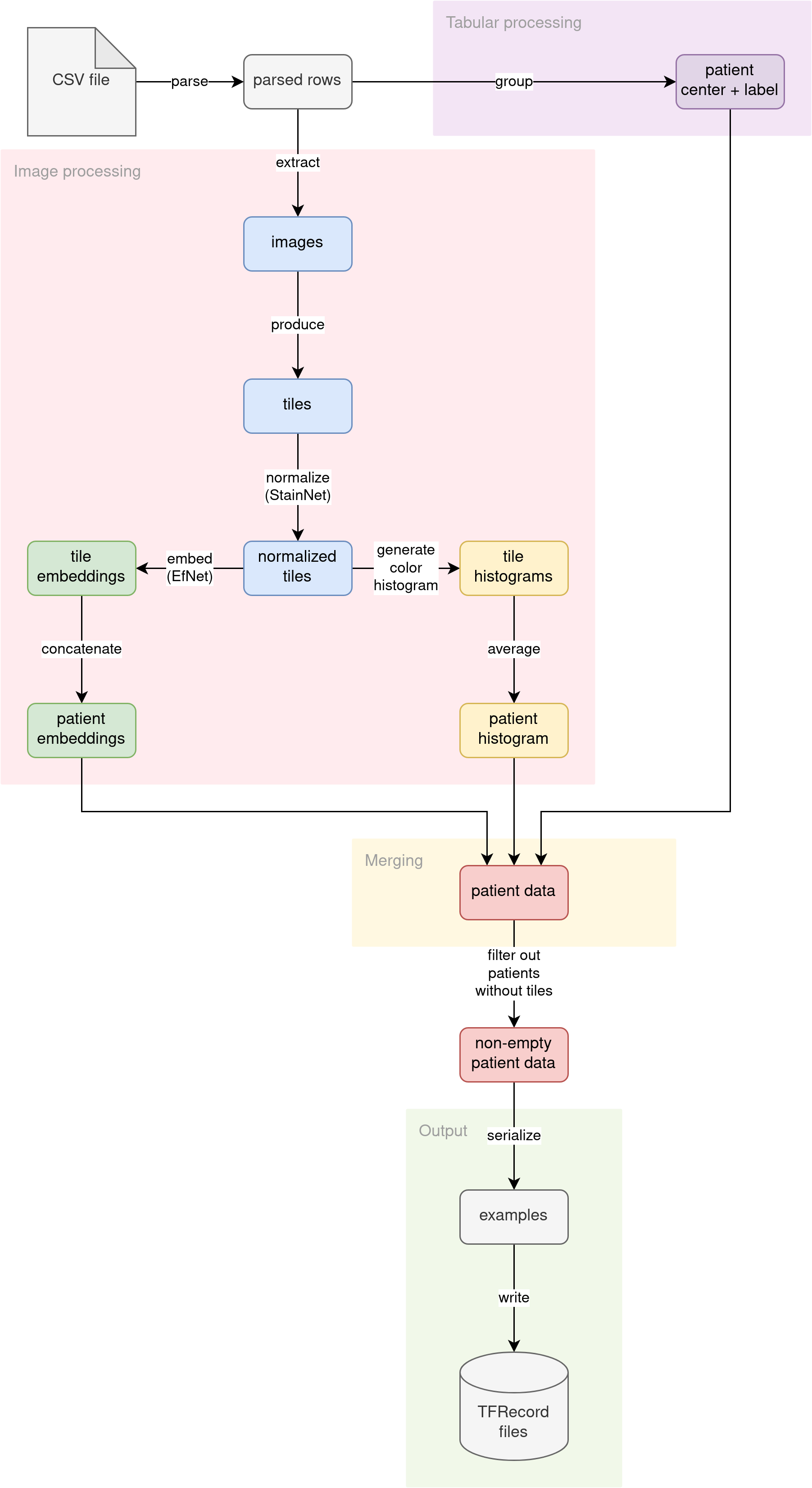
Pre-processing pipeline idea

Parse CSV

The supply CSV file (irrespective of if the coaching file with labels or the inference file with out labels) is learn into strains. The strains are then parsed into pythonic dictionaries. Affected person ID is used as the important thing. A number of photographs per affected person are usually not grouped but. This step prepares the elemental constructing block for the remainder of the pipeline.

Additional down the pipeline, processing diverges into two streams:

• Tabular information processing
• Picture information processing

Tabular information processing

The affected person tabular attributes (ID of the medical middle the place the affected person was admitted and non-obligatory analysis label) are grouped. Because the analysis is set per affected person, we’re grouping the information by affected person ID. The attributes (medical middle ID and analysis label) ought to match throughout a number of affected person photographs.

Picture information processing

The first supply of knowledge for this downside is the pictures themselves. We determined to research the pictures within the following methods:

• Cut up the picture into tiles and use tiles as enter to a pc imaginative and prescient mannequin
• Extract histograms of colours in photographs

Tile era

The uncooked TIFF enter photographs are too huge to make use of for processing straight. We determined to go along with the A number of Occasion Studying strategy, the place we feed a mannequin with a bag of zoomed-in picture tiles in order that the analysis will be made by taking a look at microscopic constructions contained in the tissue.

The tiles are going to be generated from all affected person’s photographs. There can be a single label for the entire bag. We determined to separate every uncooked enter picture into smaller tiles (448x448 pixels) and feed the following ML fashions with a set of small tiles downsized solely to half of the unique tile measurement (224x224 pixels – which means a 50% zoom stage as in comparison with the uncooked picture).

The uncooked enter photographs are giant, however they comprise intensive sections of the background. In most photographs, there may be way more background than the precise tissue. We wished to restrict additional processing to solely elements of the picture that contained strong tissue. To that finish, we filter out tiles containing an excessive amount of background.

We downscale the unique uncooked picture to make it appropriate for evaluation. Then, we divide it into tiles. For every tile, we analyze the scaled-down model and test the proportion of the tile’s pixels detected as background. Totally different photographs from the dataset have totally different background colours (not all the time pure white). 

We assumed that very vibrant pixels (over 190 on all 3 RGB channels) comprise a background. If the tile had greater than 10% pixels marked as background, we might discard it from additional processing, leaving solely tiles that comprise >90% tissue.

This strategy enabled us to generate a subset of tissue-only tiles from every picture with 50% zoom.

Tile normalization

We seen that the uncooked photographs had totally different shade schemes. Some have been pinkish, some yellowish, and others greenish. We determined to make use of StainNet to normalize all photographs earlier than additional processing. Since StainNet produces coloring constant throughout a number of tiles of the identical picture, we might apply the pre-trained StainNet Neural Community on batches of random tiles.

Tile embedding

Pc imaginative and prescient is a posh downside. Coaching Convolutional Neural Networks for picture classification is time and resource-intensive. 

As a substitute of ranging from scratch, we utilized a way referred to as switch studying by utilizing a pre-trained EfficientNet neural community to generate tile embeddings. We ran every normalized tile by way of the pre-trained EfficientNet B0 mannequin with out prime layers. The neural community generated a [7, 7, 1280]-shape embedding for every tile. 

Considering that the place of tissue construction within the tile will not be related to fixing the issue, we determined to combination the embeddings throughout the [7, 7]-shape picture to provide a single 1280-dimensional embedding vector. We generated each max and imply aggregations and left it as much as the following mannequin to choose which of these it wished to make use of as enter.

Lastly, for every affected person, we generate two vectors:

• • avg – mean-aggregated embeddings of form [<number of tiles per patient>, 1280]*

• • max – max-aggregated embeddings of form [<number of tiles per patient>, 1280]*

*the place <variety of tiles per affected person> is a ragged dimension whose measurement is determined by the variety of tiles generated per affected person.

The generated embedding vectors are a lot smaller in measurement than the unique photographs. They take up much less disk area and allow us to cache the entire dataset for extra environment friendly coaching.

Shade histograms

Considering that totally different colours of pixels within the tissue pattern correspond to totally different microscopic constructions, we found out that the proportion of given constructions per tile is perhaps an indicative diagnostic function. We determined that we might categorical the proportions by calculating shade histograms for all pixels within the picture. We generate a [16, 16, 16]-shape histogram for every normalized tile.

Since there are a number of tiles per affected person and we wished to research the general distribution of microscopic constructions, we’re averaging the histograms alongside all tiles generated from all person’s photographs. The aggregation produces a single vector of form [16, 16, 16] for a affected person. This histogram vector turns into one other enter out there to subsequent fashions.

Merging

We now have three unbiased streams of options per affected person, calculated by totally different elements of the pipeline:

• A single shade histogram (form [16, 16, 16])
• A number of tile embeddings per affected person (two aggregations, every form [<number of tiles per patient>, 1280])
• 2 tabular options (medical middle ID and non-obligatory analysis label) per affected person (every a scalar worth)

Within the merging part of preprocessing, we join all of those options right into a single entity, utilizing affected person ID because the be part of key.

Output

The pipeline converts the joined options into Tensorflow’s tf.prepare.Instances. Then, the serialized Examples are written to a set of TFRecord information. These TFRecord information can later be loaded by the mannequin coaching code or inference code as datasets. The generated datasets are a lot smaller in disk measurement than the unique uncooked photographs (from ~400 GB, we distill ~2.2 GB datasets).

To deal with the implementation of the advanced preprocessing pipeline, we used Apache Beam. Apache Beam is an open-source framework that gives a unified programming mannequin for batch and streaming information processing pipelines. 

The framework simplifies the implementation of large-scale information processing. Beam helps a big set of enter and output codecs. The processing pipeline written utilizing Apache Beam will be executed each domestically in addition to scaled up on the cloud (for instance, utilizing Dataflow on the Google Cloud Platform).

We used Apache Beam for the next causes:

• We now have a posh pipeline with three parallel streams of labor and a merging part that may be properly expressed utilizing Beam SDK
• Beam helps textual content inputs (CSV file)
• Beam helps TFRecord sinks
• Beam transparently helps Google Cloud Storage (the place we stored our information)
• Beam can run domestically, taking full benefit of multiprocessing, effectively utilizing all domestically out there processing energy (helpful for Kaggle submissions with restricted allowed run time)

Apache Beam is a constructing block of different production-ready instruments. For instance, many Tensorflow Prolonged elements use Beam underneath the hood.

Processing giant medical photographs

Dealing with giant TIFF enter photographs can’t be carried out utilizing normal Python instruments for picture loading (PIL) merely due to reminiscence constraints.

An instance RGB enter picture of measurement 46177 by 77440 pixels would take  46177 * 77440 * 3 = 10 727 840 640 bytes – nearly 11 GB! There are even greater photographs within the coaching set. When paired with Kaggle cases having 16 GB of RAM, one can simply see that loading the entire picture into reminiscence is a no-go.

As a substitute, we have to use different third-party libraries that may have the ability to function on the large TIFF photographs with out loading them entire into reminiscence. 

We used two such libraries:

• libvips – to effectively load down-scaled variations of enter photographs to carry out background evaluation
• openslide – to effectively extract solely the attention-grabbing tiles (stuffed mainly with tissue) of the unique picture in unique decision

Utilizing libvips to load down-scaled variations of enormous photographs

We determined to down-scale the enter photographs by an element of 16. For the earlier pattern picture, the reminiscence wanted to retailer the smaller model of the picture is just (46177/16) * (77440/16) * 3 = 41 940 720  bytes (lower than 42 MB, in comparison with ~11 GB for the total model).

import numpy as np
from numpy import typing as npt
import pyvips


def load_downscaled_image(
    local_file_path: str,
    downsample_ratio: int = 16,
) -> npt.NDArray[np.uint8]:
    full_img = pyvips.Picture.new_from_file(local_file_path)
    scaled_down_image: npt.NDArray[np.uint8] = full_img.resize(
        1 / downsample_ratio
    ).numpy()
    return scaled_down_image
    

Utilizing the code above,  libvips will load and downscale the picture on the fly with out loading the total model. The return worth will comprise a NumPy array of unsigned 8-bit integers with scaled picture contents.

Please notice that the  libvips API creates a picture processing pipeline. Utilizing new_from_file solely hundreds picture metadata. Identical factor with resize: no precise resizing is carried out. The constructed pipeline is executed solely in the mean time of express materialization – upon calling numpy().

Utilizing openslide to extract sure tiles from giant photographs

Within the earlier part, we described how we might load a scaled-down model of a giant picture for evaluation. Upon figuring out which sq. tiles of the picture comprise largely tissue, we wished to extract the contents of these tiles within the unique decision.

Since we wished to make use of EfficientNet B0 in later steps, we wanted the enter photographs to have 224 by 224 decision (required enter form for EfNet). We determined to load tiles twice as huge (224 * 2 = 448 pixels in measurement) for preprocessing and scale them down by an element of 2 simply earlier than embedding them utilizing EfNet.

Every RGB tile extracted would take up (224 * 2) * (224 * 2) * 3 = 602 112  bytes of reminiscence (~600 KB).

The code under exhibits how one can use openslide to load solely particular tiles from a big picture:

from typing import Tuple, Sequence, Iterable

import openslide
from PIL import Picture


def extract_tiles(
    input_image_path: str,
    non_empty_tile_indices: Sequence[Tuple[int, int]],
    tile_size: int = 224 * 2
) -> Iterable[Image]:
    measurement = (tile_size, tile_size)
    with openslide.open_slide(input_image_path) as slide:
        for row, column in non_empty_tile_indices:
            left = column * tile_size
            prime = row * tile_size
            place = (left, prime)
            # Extract the tile from the unique picture
            # in unique decision.
            tile_img = slide.read_region(
                place, 0, measurement
            ).convert("RGB")  # convert from RGBA to RGB
            yield tile_img

A tile loaded on this trend is a PIL picture. We will convert it right into a NumPy array of unsigned 8-bit integers utilizing the next:

import numpy as np
from numpy import typing as npt


img_array: npt.NDArray[np.uint8] = np.array(tile_img)

Please notice that the tile extraction snippet doesn’t materialize all of the extracted tiles. As a substitute, the perform is a generator that materializes one tile at a time. This strategy permits us to maintain reminiscence utilization low (regardless that, from some photographs, we’re extracting hundreds of tiles) and integrates properly with Apache Beam.

Making use of mannequin predictions

In our preprocessing pipeline, we’ve two locations the place we’re executing inference utilizing pre-trained fashions:

• In uncooked tile normalization (StainNet)
• In normalized tile embedding (EfficientNet)

It’s easy to implement ML inference in Apache Beam. A ModelHandler class is offered within the apache_beam.ml.inference.base package deal that may wrap an ML mannequin for inference. It’s framework-agnostic and will be utilized to any ML mannequin. 

The category is outlined as a generic:

class ModelHandler(Generic[ExampleT, PredictionT, ModelT]):
    ...

The place the kind variables have the next that means:

• ExampleT – the kind of incoming examples
• PredictionT – the kind of outgoing predictions
• ModelT – the kind of ML mannequin loaded and used for producing predictions.

To make use of the ModelHandler, one must create a category that inherits from it with concrete sorts and implement two strategies:

• load and initialize a mannequin for processing:

  def load_model(self) -> ModelT:
      ...

• run inference on a batch of examples:

  def run_inference(
      self,
      batch: Sequence[ExampleT],
      mannequin: ModelT,
      inference_args: Elective[Dict[str, Any]] = None
  ) -> Iterable[PredictionT]:
      ...

An inference wrapper outlined within the following means will be simply built-in into an Apache Beam pipeline (see pipeline implementation snippet within the following part). Beam will robotically care for batching incoming examples (it would decide the optimum batch measurement) and loading a single mannequin occasion per node.

Beneath you’ll find a snippet that exhibits find out how to apply ModelHandler to execute tile embedding utilizing EfficientNet in TensorFlow:

from typing import (
    Iterable
    NamedTuple,
    NewType,
    Sequence,
)

from apache_beam.ml.inference.base import ModelHandler
import numpy as np
from numpy import typing as npt
import tensorflow as tf


# alias sort for string affected person ID
PatientId = NewType("PatientId", str)
# alias for NumPy tile as an array
#  of 8-bit unsigned integers
Picture = npt.NDArray[np.uint8]


class TileEntry(NamedTuple):
    """Schema for a tile entry."""

    patient_id: PatientId
    picture: Picture


class Embedding(NamedTuple):
    """Schema for aggregated embeddings."""

    max_embedding: tf.Tensor
    avg_embedding: tf.Tensor


class EmbeddingEntry(NamedTuple):
    """Schema for prediction entry."""

    patient_id: PatientId
    embedding: Embedding


def embed_tiles(
    mannequin: tf.keras.Mannequin,
    tiles_batch: Sequence[Image],
) -> Iterable[Embedding]:
    """
    Run a batch of enter photographs by way of EfNet
    to generate aggregated embeddings.
    """
    # convert from NumPy to TensorFlow
    input_tensor = tf.ensure_shape(
        tf.convert_to_tensor(tiles_batch),
        [None, 224 * 2, 224 * 2, 3],
    )
    # The enter tile is twice as huge as wanted
    # for EfNet - we scaled it down 2x right here.
    resized_input_tensor = tf.picture.resize(input_tensor, [224, 224])
    # generate embeddings utilizing EfNet
    outcomes = mannequin(resized_input_tensor, coaching=False)
    avg_embeddings = tf.ensure_shape(outcomes["avg"], [None, 1280])
    max_embeddings = tf.ensure_shape(outcomes["max"], [None, 1280])
    # wrap the outcomes
    for avg_embedding, max_embedding in zip(avg_embeddings, max_embeddings):
        yield Embedding(avg_embedding=avg_embedding, max_embedding=max_embedding)


class TileEmbeddingModelHandler(
    ModelHandler[TileEntry, EmbeddingEntry, tf.keras.Model]
):
    """Wrapper round EfficientNet embedding."""

    def load_model(self) -> tf.keras.Mannequin:
        """Put together an EfNet aggregation mannequin for tile photographs."""
        # The mannequin will devour 224x224 RGB photographs
        picture = tf.keras.layers.Enter(
            form=(224, 224, 3), identify="picture", dtype=tf.float32
        )
        # We use EfNet B0 with out prime layers for embedding
        spine = tf.keras.purposes.EfficientNetB0(
            include_top=False, weights="imagenet", input_tensor=picture
        )
        # To avoid wasting on compute sources, we cannot fine-tune the EfNet spine
        spine.trainable = False
        # The spine output has form [<batch size>, 7, 7, 1280]
        # We generate two aggregations over the spine output
        # to acquire a [<batch size>, 1280] form
        avg_pool = tf.keras.layers.GlobalAveragePooling2D()(spine.output)
        max_pool = tf.keras.layers.GlobalMaxPooling2D()(spine.output)
        mannequin = tf.keras.Mannequin(
            picture, {"avg": avg_pool, "max": max_pool}, identify="EfficientNet"
        )
        mannequin.compile()
        return mannequin

    def run_inference(
        self,
        batch: Sequence[TileEntry],
        mannequin: tf.keras.Mannequin,
        inference_args: Elective[Dict[str, Any]] = None,
    ) -> Iterable[EmbeddingEntry]:
        """Run inference utilizing the loaded mannequin."""
        # Extract simply the tile photographs from the enter batch
        input_images = [tile.image for tile in batch]
        # Embed tile photographs utilizing EfNet
        embeddings = embed_tiles(mannequin, input_images)
        # Wrap the ensuing embeddings along with the affected person identifier
        for tile, embedding in zip(batch, embeddings):
            yield EmbeddingEntry(patient_id=tile.patient_id, embedding=embedding)

Pipeline implementation

Our preprocessing pipeline is relatively advanced, with a number of parallel streams of processing. If we wished to precise that in pure Python, we might find yourself with a really advanced code. Fortunately, we will use Apache Beam to outline and run the advanced pipeline comparatively simply.

Beam pipeline syntax

To create a pipeline, one wants to make use of Pipeline from apache_beam (the module is usually aliased as simply beam), ideally as a context supervisor:

with beam.Pipeline(choices=beam_options) as pipeline:
    ...

To attach operations, one makes use of the pipe operator (|):

filenames = pipeline | beam.Create([input_csv_path])
csv_dicts = filenames | beam.FlatMap(read_csv_lines)
parsed_rows = csv_dicts | beam.Map(parse_row)

Every operation can optionally get a descriptive identify (that is required if varieties of operations within the pipeline are usually not distinctive) utilizing the precise bit shift operator (>>):

filenames = pipeline | "Create" >> beam.Create([input_csv_path])
csv_dicts = filenames | "ParseCSV" >> beam.FlatMap(read_csv_lines)
parsed_rows = csv_dicts | "ParseRows" >> beam.Map(parse_row)

The pipeline have to be comprised of Beam transforms personalized with customized callbacks (see Beam Programming Information).

Beam can learn information from totally different sources. In our pipeline, we use the Create operation to import a knowledge seed into our Beam pipeline. The op creates a assortment that may be additional processed.

Parts processed with a Beam pipeline will be of any serializable sort. Beam can use tuples as keyed components, the place the primary component of the tuple is taken into account to be the key. Keys are helpful for combining components or becoming a member of collections.

In our pipeline, we use the next Beam ops:

• Create – import static entries into Beam pipeline as a Beam assortment,
• FlatMap – map objects within the enter assortment utilizing callback the place every enter component maps to zero or many output components (useful in implementing fan-out operations or filtering),
• FlatMapTuple – like FlatMap, however the signature of the callback has the component unpacked,
• Reshuffle – artificial grouping and ungrouping that forestalls surrounding transforms from fusing (helpful to extend the parallelism of pipeline ops, particularly after fan-out operations),
• Map – map objects within the enter assortment utilizing callback the place every enter component maps to precisely one output component,
• MapTuple – like Map however the signature of the callback has the component unpacked,
• CombinePerKey – combination components that share a typical key,
• RunInference – carry out ML mannequin inference utilizing offered ModelHandler,
• CoGroupByKey – be part of components from a number of collections collectively utilizing component keys,
• Filter – filter components based mostly on a callback predicate,
• WriteToTFRecord – retailer components in a set of TFRecord information.

Pipeline definition

Pre-processing pipeline idea

Beneath you’ll find the definition of our pipeline expressed utilizing Apache Beam. You’ll be able to evaluate it with the pipeline idea diagram to find out how the a number of work streams are carried out.

from pathlib import Path
from typing import Elective

import apache_beam as beam
import tensorflow as tf
from apache_beam.ml.inference.base import RunInference
from apache_beam.choices.pipeline_options import PipelineOptions


def run_pipeline(
    *,
    input_csv_path: str,
    tiff_files_location: Path,
    output_prefix: str,
    temporary_storage_location: str,
    max_tiles: Elective[int] = None
) -> None:
    """
    Set off preprocessing pipeline.

    A CSV file guides execution. Every row within the CSV file corresponds to
    a single picture in a given storage location.
    The pipeline will produce a set of sharded TFRecord information
    that comprises an entire dataset that has affected person tile embeddings
    already grouped.
    """
    beam_options = PipelineOptions(
        runner="DirectRunner",
        direct_num_workers=0,
        direct_running_mode="multi_processing",
    )

    with beam.Pipeline(choices=beam_options) as pipeline:
        filenames = pipeline | "Create" >> beam.Create([input_csv_path])
        csv_dicts = (
            filenames
            | "ParseCSV" >> beam.FlatMap(read_csv_lines)
            | "ReshuffleLines" >> beam.Reshuffle()
        )
        parsed_rows = csv_dicts | "ParseRows" >> beam.Map(parse_row)
        keyed_rows = parsed_rows | "KeyRows" >> beam.Map(key_csv_row)

        patient_data = keyed_rows | "GroupPatientData" >> beam.CombinePerKey(
            PatientDataCombineFn()
        )

        raw_tiles = (
            keyed_rows
            | "SelectImageId" >> beam.MapTuple(select_image_id)
            | "ProduceTiles"
            >> beam.FlatMapTuple(produce_tiles, tiff_files_location, max_tiles)
        )

        normalized_tiles = raw_tiles | "NormalizeTiles" >> RunInference(
            TileNormalizationModelHandler()
        )
        embeddings = (
            normalized_tiles
            | "EmbedTiles" >> RunInference(TileEmbeddingModelHandler())
            | "CombineEmbeddings"
            >> beam.CombinePerKey(
                CombineEmbeddingsFn(
                    temporary_storage_location=temporary_storage_location
                )
            )
        )

        color_histograms = (
            normalized_tiles
            | "ComputeColorHistograms" >> beam.Map(compute_color_histogram)
            | "CombineColorHistograms" >> beam.CombinePerKey(ColorHistogramCombineFn())
        )

        merged_data = (
            {
                "patient_data": patient_data,
                "embedding": embeddings,
                "color_histogram": color_histograms,
            }
            | "MergeData" >> beam.CoGroupByKey()
            | "DropNoTiles" >> beam.Filter(has_embedding)
        )

        examples = merged_data | "ToTFExample" >> beam.MapTuple(to_example)

        examples | "WriteTFRecords" >> beam.io.tfrecordio.WriteToTFRecord(
            file_path_prefix=output_prefix,
            file_name_suffix=".tfrecord",
            coder=beam.coders.ProtoCoder(tf.prepare.Instance),
        )

For brevity, we omit the signatures of callbacks used contained in the pipeline.

Operating the pipeline

A Beam pipeline is not going to obtain excessive parallelism with default settings on a neighborhood surroundings. Apache Beam is designed to run in many various environments (Apache Flink, Spark, Google Cloud Dataflow, AWS KDA). 

The precept of Beam is write as soon as, run anyplace, so the identical pipeline is usable each on multi-machine cloud setups and domestically. Operating Beam on something other than the native machine is exterior the scope of this text. For the Kaggle competitors submission, we needed to preprocess our information on the offered Kaggle occasion that had a severed web connection.

Native Beam runner has many modes of operation that the developer can configure. For max parallelism, we used the multiprocessing operating mode. On this mode, every Beam employee would spawn a brand new Python course of that processes separate chunks of knowledge. The variety of staff auto-configured to match the variety of CPUs out there on the machine:

beam_options = PipelineOptions(
    runner="DirectRunner",
    direct_num_workers=0,
    direct_running_mode="multi_processing",
)

Please notice that Beam tries to restrict IPC (inter-process communication) bottlenecks by striving to maintain chunks of knowledge on the identical employee over a number of transforms. This habits may restrict parallelism, particularly in fan-out situations.

Fan-out is a state of affairs the place one op transforms a single enter component into many output components. That’s the case with our preliminary CSV parsing, the place from a single CSV file path (imported into the pipeline utilizing Create), we generate a whole lot of strains (utilizing FlatMap).

In a fan-out state of affairs Beam may maintain all fan-out operation’s output components on the unique employee and execute additional transformations on the output components there. Meantime different staff are idle. Please notice that this habits of Beam is wise – Beam can’t inform whether or not a given operation will find yourself as a fan-out state of affairs. Fusing transforms onto a single employee makes excellent sense in balanced situations.

The developer can affect the fusing of operations by developing the pipeline in a particular means. In our instance, we used the Reshuffle operation to forestall fusing and to make sure excessive throughput by way of parallelism after the fan-out op.

Summing up the competitors

The Mayo Clinic STRIP AI competitors posed a major problem in preprocessing the information earlier than even trying to coach an ML mannequin, given the character of the enter information (big TIFF photographs) and the submission’s technical necessities (submission time restrict and VM occasion parameters).

We might deal with the large enter photographs because of utilizing libvips and openslide libraries. Due to Apache Beam, we might additionally outline a posh preprocessing pipeline with relative ease. Beam enabled us to run our pipeline effectively, taking full benefit of the offered VM occasion to complete processing throughout the competitors’s run-time restrict (throughout submission, the pipeline preprocessed the hidden take a look at set of ~280 photographs in ~6 hours).

AI in medical imaging: the place is it helpful?

This text has proven you find out how to overcome a few of the technical challenges of utilizing AI in medical imaging, however have you learnt the place you possibly can harness the strategy we’ve defined? 

Beneath you’ll discover a number of examples.

1. Detecting breast most cancers

Breast most cancers is the second most typical most cancers amongst ladies. However typical mammogram screenings miss 1-in-5 circumstances. In accordance with a paper printed in The American Journal of Surgical Pathology, Google’s AI powered Lymph Node Assistant (LYNA) detects breast most cancers metastasis with 99% accuracy.

2. Prescribing targetted therapies

In accordance with analysis, two skilled pathologists will solely agree on a course of remedy about 60 % of the time, even when assessing the identical information. Utilizing AI in medical imaging removes subjectivity with a quantitative strategy, serving to determine the kind of most cancers and decide find out how to deal with it. With this development in precision medication, physicians can present extra customized remedy plans that focus on the particular sickness.

3. Predicting the chance of a coronary heart assault

AI in medical imaging isn’t solely useful in figuring out current circumstances. It will probably detect the chance of creating a future sickness. One latest research exhibits how combining AI imaging with scientific information helps physicians enhance predictive fashions that point out whether or not a affected person is at a excessive threat of getting a coronary heart assault.

4. Recognizing neurological decline

MRI scans support the analysis of neurological circumstances like Alzheimer’s and a number of sclerosis by serving to medical doctors spot indicators of illness, together with lesions, development, and shrinkage. Nonetheless, slight adjustments within the mind are simple for the human eye to overlook. Then again, synthetic intelligence can quantify adjustments in a affected person’s mind, permitting the early detection and analysis of neurological illness.

5. Enhancing the end result of surgical procedure

AI in medical imaging may even allow surgeons to enhance surgical outcomes. It does this by serving to healthcare professionals higher plan procedures earlier than the precise operation, decreasing surgical procedure time and main to higher outcomes.

Implement AI in your healthcare firm

Synthetic intelligence has all kinds of purposes in medication. 

And as you possibly can see, it’s advancing healthcare in a number of methods. However if you wish to study extra concerning the healthcare business’s challenges, in addition to how AI is actively fixing them, you must give our latest webinar on how healthcare corporations can create new enterprise fashions utilizing AI a watch.

Or, in case you’d like assist with medical picture processing, be happy to contact us straight. Our staff has its roots in healthcare, and we’d be delighted to share our expertise with you.