Deep Learning Fundamentals Handbook – What You Must Know to Begin Your Profession in AI

If you need to get into the sector of Artificial Intelligence (AI), probably the most in-demand profession paths nowadays, you have come to the precise place.

Learning Deep Learning Fundamentals is your important first step to studying about Computer Vision, Natural Language Processing (NLP), Large Language Models, the artistic universe of Generative AI, and extra.

If you might be aspiring Data Scientist, AI Researcher, AI Engineer, or Machine Learning Researcher, this information is made for you.

AI Innovation is occurring shortly. Whether you are newbie otherwise you’re already in Machine studying, it’s best to proceed to solidify your data base and be taught the basics of Deep Learning.

Think of this handbook as your private roadmap to navigating the AI panorama. Whether you are a budding fanatic inquisitive about how AI is reworking our world, a scholar aiming to construct a profession in tech, or knowledgeable looking for to pivot into this thrilling subject, it will likely be helpful to you.

This information might help you to:

• Learn all Deep Learning Fundamentals in a single place from scratch
• Refresh your reminiscence on all Deep Learning fundamentals
• Prepare on your upcoming AI interviews.

Table of Contents

1. Chapter 1: What is Deep Learning?
2. Chapter 2: Foundations of Neural Networks
   – Architecture of Neural Networks
   – Activation Functions
3. Chapter 3: How to Train Neural Networks
   – Forward Pass – math derivation
   – Backward Pass – math derivation
4. Chapter 4: Optimization Algorithms in AI
   – Gradient Descent – with Python  
   – SGD – with Python  
   – SGD Momentum – with Python  
   – RMSProp – with Python  
   – Adam – with Python  
   – AdamW – with Python
5. Chapter 5: Regularization and Generalization
   – Dropout
   – Ridge Regularization (L2 Regularization)
   – Lasso Regularization (L1 Regularization)
   – Batch Normalization
6. Chapter 6: Vanishing Gradient Problem
   – Use acceptable activation capabilities
   – Use Xavier or He Initialization
   – Perform Batch Normalization
   – Adding Residual Connections
7. Chapter 7: Exploding Gradient Problem
8. Chapter 8: Sequence Modeling with RNNs & LSTMs
   – Recurrent Neural Networks (RNN) Architecture
   – Recurrent Neural Network Pseudocode
   – Limitations of Recurrent Neural Network
   – Long Short-Term Memory (LSTM) Architecture
9. Chapter 9: Deep Learning Interview Preparation
   – Part 1: Deep Learning Interview Course [50 Q&A]
   – Part 2: Deep Learning Interview Course [100 Q&A]

Prerequisites

Deep Learning is a sophisticated research space inside the fields of Artificial Intelligence and Machine Learning. To totally grasp the ideas mentioned right here, it is important that you’ve a stable basis in a number of key areas.

1. Machine Learning Basics

Understanding the core ideas of machine studying is essential. If you are not but conversant in these, I like to recommend trying out my Fundamentals of Machine Learning Handbook, the place I’ve laid out all the required groundwork. Also, my Fundamentals of Machine Learning course gives complete educating on these ideas.

2. Fundamentals of Statistics

Statistics play an important function in making sense of information patterns and inferences in machine studying. For those that must brush up on this, my Fundamentals of Statistics course is a one other useful resource the place I cowl all of the important statistical ideas you may want.

3. Linear Algebra and Differential Theory

A excessive stage understanding of linear algebra and differential concept can also be essential. We’ll cowl some points, akin to differentiation guidelines, on this handbook. We’ll go over matrix multiplication, matrix and vector operations, normalization ideas, and the fundamentals of differentiation concept.

But I encourage you to strengthen your understanding in these areas. More on this content material you’ll find on freeCodeCamp when trying to find “Linear Algebra” like this course “Full Linear Algebra Course“.

Note that if you do not have the stipulations akin to Fundamentals of Statistics, Machine Learning, and Mathematics, following together with this handbook can be fairly a problem. We’ll use ideas from all these areas together with the imply, variance, chain guidelines, matrix multiplication, derivatives, and so forth. So, please be sure you have these to take advantage of out of this content material.

Referenced Example – Predicting House Price

Throughout this guide, we can be utilizing a sensible instance for instance and make clear the ideas you are studying. We will discover this concept of predicting a home’s value based mostly on its traits. This instance will function a reference level to make the summary or complicated ideas extra concrete and simpler to grasp.

Chapter 1: What is Deep Learning?

Deep Learning is a sequence of algorithms impressed by the construction and performance of the mind. Deep Learning permits quantitative fashions composed of a number of processing layers to check the information illustration with a number of ranges of abstraction.

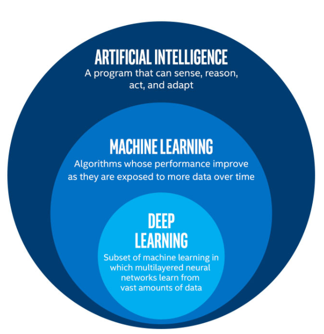
Deep Learning is a department of Machine Learning, and it tries to imitate the way in which the human mind works and makes choices based mostly on neural network-based fashions.

In less complicated phrases, Deep Learning is extra superior and extra complicated model of conventional Machine Learning. Deep Learning Models are based mostly on Neural Networks they usually attempt to mimic the way in which people assume and make choices.

The downside with conventional Statistical or ML strategies is that they’re based mostly on particular guidelines and directions. So, each time the set of mannequin assumptions will not be glad, the mannequin can have very arduous time to unravel the issue and carry out prediction. There are additionally varieties of issues akin to picture recognition, and different extra superior duties, that may’t be solved with conventional Statistical or Machine Learning fashions.

Here is mainly the place Deep Learning is available in.

Applications of Deep Learning

Here are some examples the place Deep Learning is used throughout numerous industries and purposes:

Healthcare

• Disease Diagnosis and Prognosis: Deep studying algorithms assist to research medical photos like X-rays, MRIs, and CT scans to diagnose illnesses akin to most cancers extra precisely  with laptop imaginative and prescient fashions. They do that way more shortly than conventional strategies. They can even predict affected person outcomes by analyzing patterns in affected person information.
• Drug Discovery and Development: Deep Learning fashions assist in figuring out potential drug candidates and rushing up the method of drug growth, considerably lowering time and prices.

Finance

• Algorithmic Trading: Deep studying fashions are used to foretell inventory market tendencies and automate buying and selling choices, processing huge quantities of monetary information at excessive velocity.
• Fraud Detection: Banks and monetary establishments make use of deep studying to detect uncommon patterns indicative of fraudulent actions, thereby enhancing safety and buyer belief.

Automotive and Transportation

• Autonomous Vehicles: Self-driving vehicles additionally use deep studying closely to interpret sensor information, permitting them to navigate safely in complicated environments, utilizing laptop imaginative and prescient and different strategies.
• Traffic Management: AI fashions analyze visitors patterns to optimize visitors circulation and scale back congestion in cities.

Retail and E-Commerce

• Personalized Shopping Experience: Deep studying algorithms assist in retail and E-Commerce to research buyer information and supply personalised product suggestions. This enhances the consumer expertise and boosts gross sales.
• Supply Chain Optimization: AI fashions forecast demand, optimize stock, and improve logistics operations, bettering effectivity within the provide chain.

Entertainment and Media

• Content Recommendation: Platforms like Netflix and Spotify use deep studying to research consumer preferences and viewing historical past to advocate personalised content material.
• Video Game Development: AI is used to create extra real looking and interactive gaming environments, enhancing participant expertise.

Technology and Communications

• Virtual Assistants: Siri, Alexa, and different digital assistants use deep studying for pure language processing and speech recognition, making them extra responsive and user-friendly.
• Language Translation Services: Services like Google Translate leverage deep studying for real-time, correct language translation, breaking down language obstacles.

Manufacturing and Production

• Predictive Maintenance: Deep studying fashions predict when machines require upkeep, lowering downtime and saving prices.
• Quality Control: AI algorithms examine and detect defects in merchandise at excessive velocity with larger accuracy than human inspectors.

Agriculture

• Crop Monitoring and Analysis: AI fashions analyze drone and satellite tv for pc imagery to observe crop well being, optimize farming practices, and predict yields.

Security and Surveillance

• Facial Recognition: Used for enhancing safety methods, deep studying fashions can precisely determine people even in crowded environments.
• Anomaly Detection: AI algorithms monitor safety footage to detect uncommon actions or behaviors, aiding in crime prevention.

Research and Academia

• Scientific Discovery: Deep studying assists researchers in analyzing complicated information, resulting in discoveries in fields like astronomy, physics, and biology.
• Educational Tools: AI-driven tutoring methods present personalised studying experiences, adapting to particular person scholar wants.

Deep Learning has drastically refined state-of-the-art speech recognition, object recognition, speech comprehension, automated translation, picture recognition, and lots of different disciplines akin to drug discovery and genomics.

Chapter 2: Foundations of Neural Networks

Now let’s speak about some key traits and options of Neural Networks:

• Layered Structure: Deep studying fashions, at their core, encompass a number of layers, every reworking the enter information into extra summary and composite representations.
• Feature Hierarchy: Simple options (like edges in picture recognition) recombine from one layer to the following, to kind extra complicated options (like objects or shapes).
• End-to-End Learning: DL fashions carry out duties from uncooked information to ultimate classes or choices, typically bettering with the quantity of information offered. So, giant information performs ket function for Deep Learning.

Here are the core elements of Deep Learning fashions:

Neurons

These are the essential constructing blocks of neural networks that obtain inputs and cross on their output to the following layer after making use of an activation perform (extra on this within the following chapters).

Weights and Biases

Parameters of the neural community which might be adjusted via the educational course of to assist the mannequin make correct predictions. These are the values that the optimization algorithm ought to constantly optimize ideally in brief period of time to achieve probably the most optimum and correct mannequin (for instance, generally referenced by w_ij and b_ij ).

Bias Term: In follow, a bias time period ( b ) is commonly added to the input-weight product sum earlier than making use of the activation perform. This is a time period that allows the neuron to shift the activation perform to the left or proper, which might be essential for studying complicated patterns.

Learning Process: Weights are adjusted throughout the community’s coaching section. Through a course of typically involving gradient descent, the community iteratively updates the weights to attenuate the distinction between its output and the goal values.

Context of Use: This neuron may very well be half of a bigger community, consisting of a number of layers. Neural networks are employed to sort out an enormous array of issues, from picture and speech recognition to predicting inventory market tendencies.

Mathematical Notation Correction: The equation offered within the textual content makes use of the image ( phi ), which is unconventional on this context. Typically, a easy summation ( sum ) is used to indicate the aggregation of the weighted inputs, adopted by the activation perform ( f ), as in

$$
fleft(sum_{i=1}^{n} W_ix_i + shiny)
$$

Activation Functions

Functions that introduce non-linear properties to the community, permitting it to be taught complicated information patterns. Thanks to activation capabilities, as a substitute of appearing as of all enter indicators or hidden models are equally essential, activation capabilities assist to rework the these values, which ends as a substitute of linear kind of mannequin to a non-linear way more versatile mannequin.

Each neuron in a hidden layer transforms inputs from the earlier layer with a weighted sum adopted by a non-linear activation perform (that is what differentiates your non-linear versatile neural community from widespread linear regression). The outputs of those neutrons are then handed on to the following layer and the following one, and so forth, till the ultimate layer is achieved.

We will talk about activation capabilities intimately on this handbook, together with the examples of 4 hottest activation capabilities to make this very clear because it’s essential idea and is essential a part of studying course of in neural networks.

This technique of inputs going via hidden layers utilizing activation perform(s) and leading to an output is named ahead propagation.

Architecture of Neural Networks

Neural community often have three varieties of layers: enter layers, hidden layers, and output layers. Let’s be taught a bit extra about every of those now.

We’ll use our home value prediction instance to be taught extra about these layers. Below you may see the determine visualizing a easy neural community architetcure which we’ll unpack layer by layer.

Input layers

Input layers are the preliminary layers the place the information is. They comprise the options that your mannequin takes in as enter to then practice your mannequin.

This is the place the neural community receives its enter information. Each neuron within the enter layer of your neural community represents a function of the enter information. If you’ve got two options, you should have two enter layers.

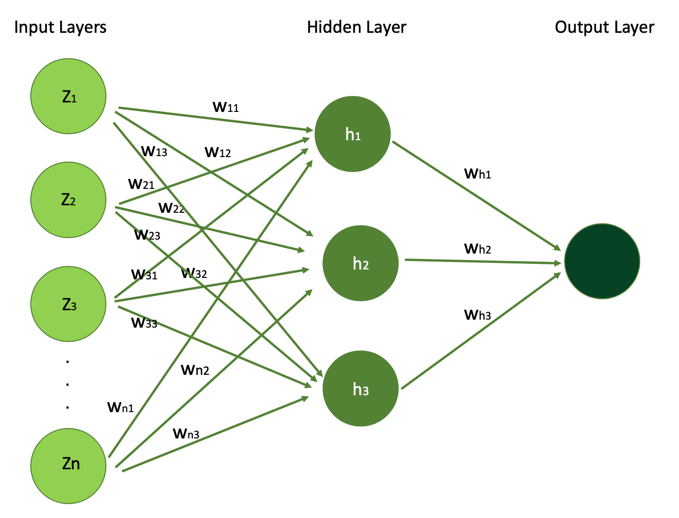
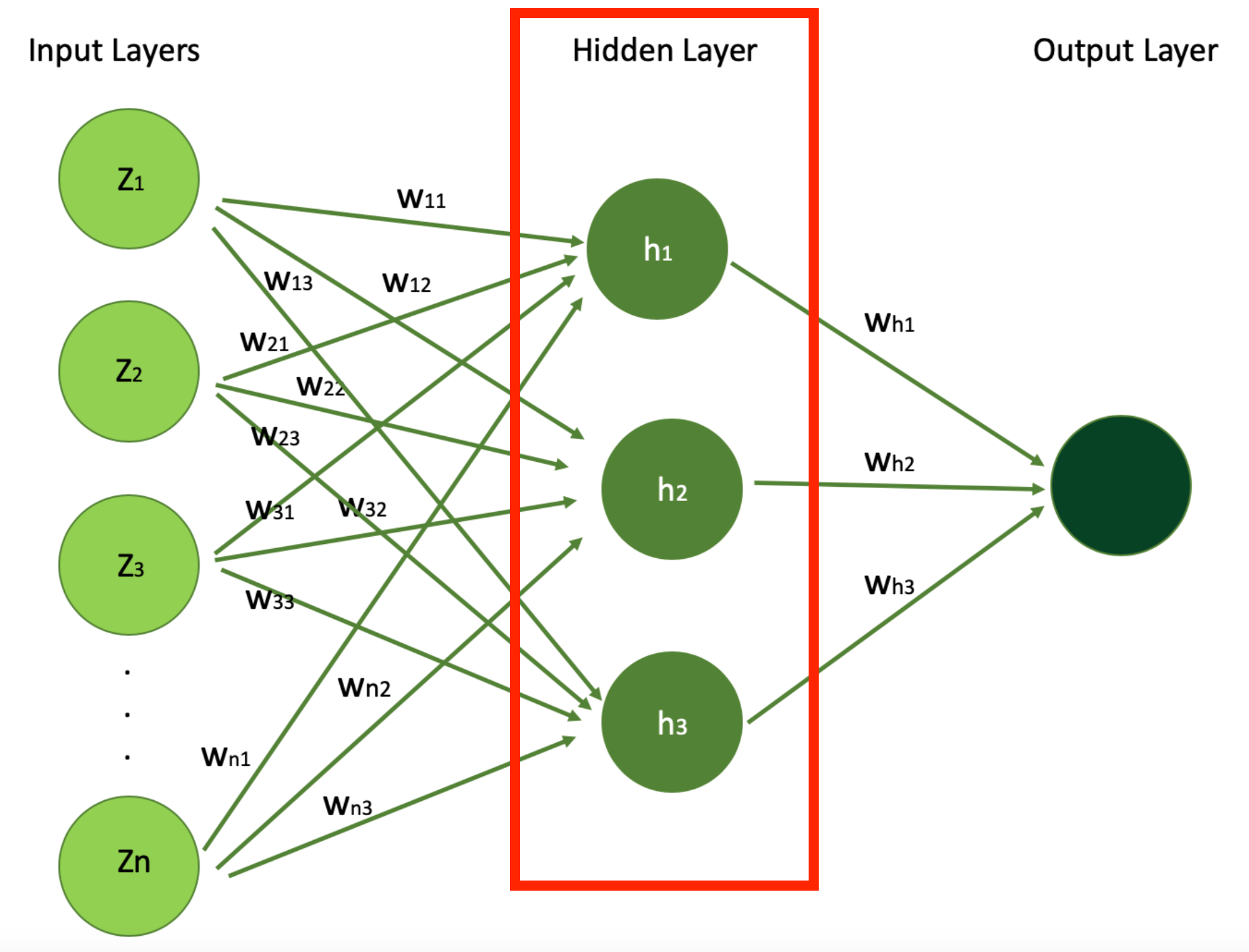
Below is the visualization of structure of easy Neural Network, with N enter options (N enter indicators) which you’ll see within the enter layer. You can even see the only hidden layer with 3 hidden models h1,h2, and h3 and the output layer.

Let’s begin with Input Layer and perceive what are these Z1, Z2, … , Zn options.

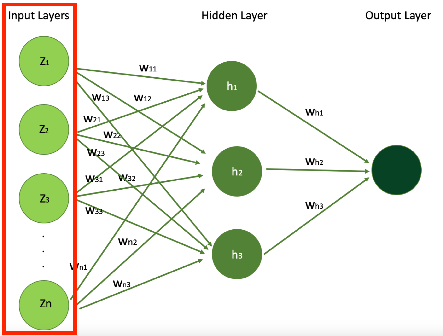
In our instance of utilizing neural networks for predicting a home’s value, the enter layer will take home options such because the variety of bedrooms, age of the home, proximity to the ocean, or whether or not there is a swimming pool, with the intention to study the home. This is what can be given to the enter layer of the neural community. Each of those options serves as an enter neuron, offering the mannequin with important information.

But then there’s the query of how a lot every of those options ought to contribute to the educational course of. Are all of them equally essential, or some are extra essential and may contribute extra to the estimation of the value?

The reply to this query lies in what we’re calling “weights” that we outlined earlier together with bias components.

In the determine above, every neuron will get weight w_ij the place i is the enter neuron index and j is the index of the hidden unit they contribute within the Hidden Layer. So, for instance w_11, w_12, w_13 describe how a lot function 1 is essential for studying about the home for hidden unit h1, h2, and h3 respectively.

Keep these weight parameter in thoughts as they’re probably the most essential components of a neural community. They are the significance weights that the neural community can be updating throughout coaching course of, with the intention to optimize the educational course of.

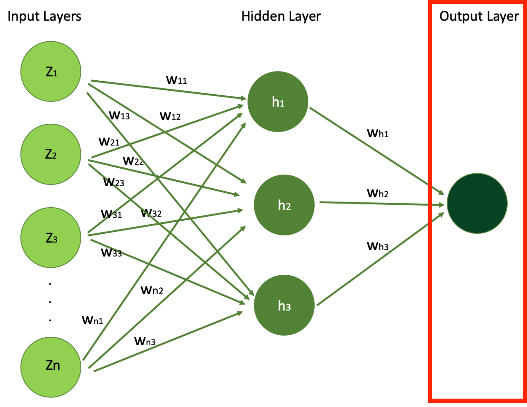
Hidden layers

Hidden layers are the center a part of your mannequin the place studying occurs. They come proper after Input Layers. You can have from one to many hidden layers.

Let’s simplify this idea by our easy neural community together with our home value instance.

Below, I highlighted the Hidden Layer in our merely neural community whose structure we noticed earlier, which you’ll consider as a vital half in your neural community to extract patterns and relationships from the information that aren’t instantly obvious from the primary view.

In our instance of estimating a home’s value with a neural community, the hidden layers play an important function in processing and deciphering the knowledge acquired from the enter layer, like the home options we simply talked about above.

These layers encompass neurons that apply weights and biases to the enter options – like home age, variety of bedrooms, proximity to the ocean, and the presence of a swimming pool – to extract patterns and relationships that aren’t instantly obvious.

In this context, hidden layers may be taught complicated interdependencies between home options, akin to how the mix of a first-rate location, home age and trendy facilities considerably boosts the value of the home.

They act because the neural community’s computational engine, reworking uncooked information into insights that result in an correct estimation of a home’s market worth. Through coaching, the hidden layers regulate these weights and biases (parameters) to attenuate fashions prediction errors, steadily bettering the mannequin’s accuracy in estimating home costs.

These layers carry out the vast majority of the computation via their interconnected neurons. In this straightforward instance, we have only one hidden layer, and three hidden models (for instance, one other hyperparameter to optimize throughout your studying utilizing methods akin to Random Search CV or others).

But in actual world issues, neural networks are a lot deeper and your variety of hidden layers, with the weights and bias parameters, can exceed billions with many hidden layers.

Output layer

Output layers are the ultimate element of a neural community – the ultimate layer which gives the output of the neural community after all of the transformations into output for particular single activity. This output might be single worth (in regression case for instance) or a vector (like in giant language fashions had been we produce vector of chances, or embeddings).

An output layer could be a class label for a classification mannequin, a steady numeric worth for regression mannequin, or perhaps a vector of numbers, relying on the duty.

Hidden layers in neural community are the place the precise studying occurs, the place the deep studying community learns from the information by extracting and reworking the offered options.

As the information goes deeper into the community, the options turn into extra summary and extra composite, with every layer constructing on the earlier layers output/values. The depth and the width (variety of neurons) of hidden layers are key components within the community’s capability to be taught complicated patterns. Below is the digram we noticed earlier than showcasing the structure of easy neural networks.

In our instance of home value prediction, the end result of the educational course of is represented by the output layer, which represents our ultimate objective: the anticipated home value.

Once the enter options – just like the variety of bedrooms, the age of the home, distance to the ocean, and whether or not there is a swimming pool – are fed into the neural community, they journey via a number of hidden layers of neural community. It’s inside these hidden layers that neural community discovers complicated patterns and interconnections inside the information.

Finally, this processed info reaches the output layer, the place the mannequin consolidates all its findings and produces the ultimate outcomes or predictions, on this case the home value.

So, the output layer consolidates all of the insights gained. These transformations are utilized all through the hidden layers to supply a single worth: the anticipated value of the home (typically referred to by Y^, pronounced “Y hat”).

This prediction is the neural community’s estimation of the home’s market worth, based mostly on its realized understanding of how totally different options of the home have an effect on the home value. It demonstrates the community’s means to synthesize complicated information into actionable insights, on this case, producing an correct value prediction, via its optimized mannequin.

Activation capabilities

Activation capabilities introduce non-linear properties to the neural community mannequin, which allows the mannequin to be taught extra complicated patterns.

Without non-linearity, your deep community would behave identical to a single-layer perceptron, which might solely be taught linear separable capabilities. Activation capabilities outline how the neurons needs to be activated – therefore the title activation perform.

Activation capabilities function the bridge between the enter indicators acquired by the community and the output it generates. These capabilities decide how the weighted sum of enter neurons – every representing a selected function just like the variety of bedrooms, home age, proximity to the ocean, and presence of a swimming pool – needs to be remodeled or “activated” to contribute to the community’s studying course of.

Activation capabilities are an especially essential a part of coaching Neural Nets. When the online consists of Hidden Layers and Output Layers, it’s essential to choose an activation perform for each of them (totally different activation capabilities could also be utilized in totally different components of the mannequin). The alternative of activation perform has a big impact on the neural networks’ efficiency and functionality.

Each of the incoming indicators or connections are dynamically strengthened or weakened based mostly on how typically they’re used (that is how we be taught new concepts and ideas). It is the energy of every connection that determines the contribution of the enter to the neurons’ output.

After being weighted by the energy of their respective indicators, the inputs are summed collectively within the cell physique. This is then remodeled into a brand new sign that’s transmitted or propagated alongside the cells’ axon and despatched off to different neurons. This practical work of activation perform can mathematically be represented as follows:

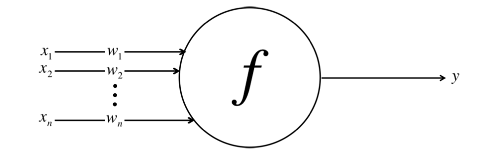
Here we now have inputs x1, x2, …xn and their corresponding weights w1, w2, … wn, and we combination them into single worth of Y by utilizing activation perform f.

This determine is a simplified model of a neuron inside a man-made neural community. Each enter ( X_i ) is related to a corresponding weight ( W_i ), and these merchandise are aggregated to compute the output ( Y ) of the neuron. The X_i is the enter worth of sign i (just like the variety of bedrooms of the home, as a function describing the home). Its significance weight by w_i corresponds to every X_i, so the sum of all these weighted enter values might be expressed as follows:

$$
phileft(sum_{i=1}^{m} w_i x_iright)

$$

In this equation, phi represents the perform we use to affix indicators from totally different enter neurons into one worth. This perform is known as the Activation Function.

Each synapse will get assigned a weight, an significance worth. These weights and biases kind the cornerstone of how Neural Networks be taught. These weights and biases decide whether or not the indicators get handed alongside or not, or to what extent every sign will get handed alongside.

In the context of predicting home costs, after the enter options are weighted based on their relevance realized via coaching, the activation perform comes into play. It takes this weighted sum of inputs and applies a selected mathematical operation to supply an activation rating.

This rating is a single worth that effectively represents the aggregated enter info. It allows the community to make complicated choices or predictions based mostly on the enter information it receives.

Essentially, activation capabilities are the mechanism via which neural networks convert an enter’s weighted sum into an output that is sensible within the context of the precise downside being solved (like estimating a home’s value right here). They enable the community to be taught non-linear relationships between options and outcomes, enabling the correct prediction of a home’s market worth from its traits.

The trendy default or hottest activation perform for hidden layers is the Rectifier Linear Unit (ReLU) or Softmax perform, primarily for accuracy and efficiency causes. For the output layer, the activation perform is especially chosen based mostly on the format of the predictions (likelihood, scaler, and so forth).

Whenever you might be contemplating any activation perform, concentrate on the Vanishing Gradient Problem (we’ll revisit this subject later). This occurs when gradients are too small or too giant, they will make the educational course of troublesome.

Some activation capabilities like sigmoid or tanh may cause vanishing gradients in deep networks whereas a few of them might help mitigate this situation.

Let’s take a look at just a few other forms of activation capabilities now, and when/how they’re helpful.

Linear Activation Function

A Linear Activation Function might be expressed as follows:

$$
f(z) = z
$$

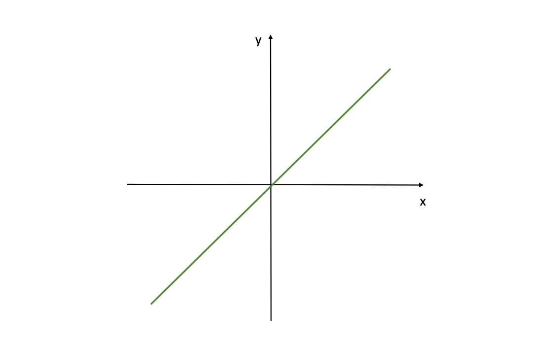
This grapgh reveals a linear activation perform for a neural community, outlined by f(z)=z.  Where z is the enter (referred to as Z-scores as we talked about earlier than) for the activation perform f( ). This means the output is immediately proportional to the enter.

Linear Activation Functions are the only activation capabilities, they usually’re comparatively simple to compute. But they’ve an essential limitation: NNs with solely linear neurons might be expressed as a community with no hidden layers – however the hidden layers in NNs are what allows them to be taught essential options from enter indicators.

So, with the intention to be taught complicated patterns from complicated issues, we’d like extra superior Activation Functions slightly than Linear Functions.

You can use a linear perform, as an example, within the final output layer when the plain end result is sweet sufficient for you and also you don’t need any transformation. But 99% of the time this activation perform is ineffective in Deep Learning.

Sigmoid Activation Function

One of the preferred activation capabilities is the Sigmoid Activation Function, which might be expressed as follows:

$$
f(z) = frac{1}{1 + e^{-z}}
$$

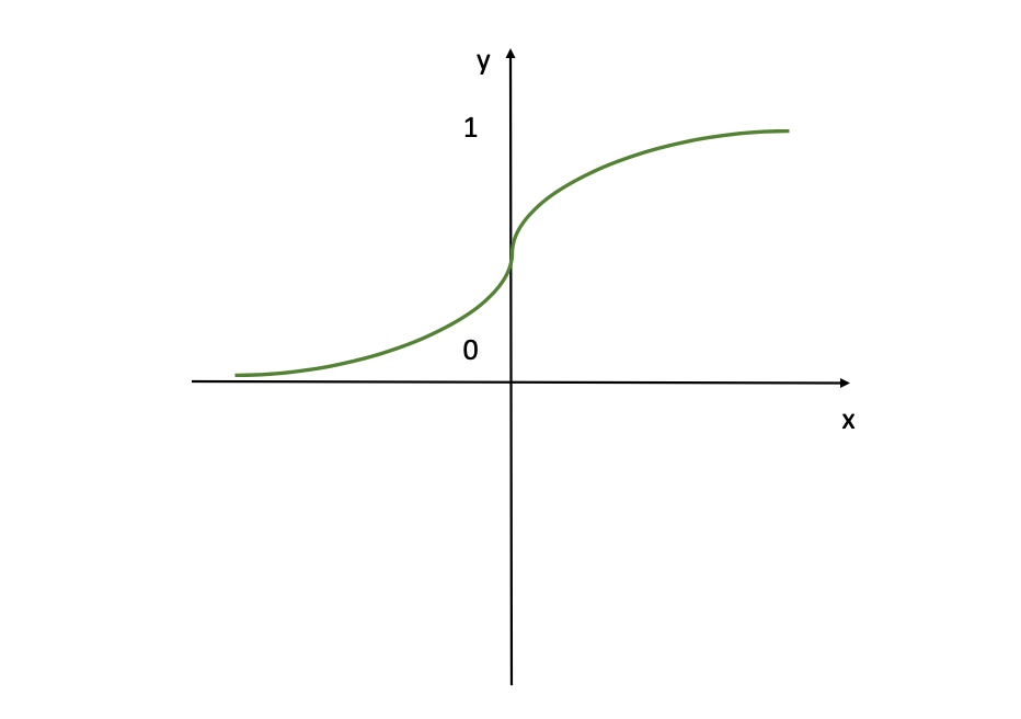
In this determine the  sigmoid activation perform is visualised, which is a easy, S-shaped curve generally utilized in neural networks. If you might be conversant in Logistic Regression, then this perform will appear acquainted to you as nicely. This perform transforms all enter values to values within the vary of (0,1) which may be very handy if you need the mannequin to supply output within the type of chances or a %.

Basically, when the logit may be very small, the output of a logistic neuron may be very near 0. When the logit may be very giant, the output of the logistic neuron is nearer to 1. In-between these two excessive values, the neuron assumes an S-shape.  This S-shape of the curve additionally helps to distinguish between outputs which might be near 0 or near 1, offering a transparent determination boundary.

You’ll typically use the Sigmoid Activation Function within the output layer, because it’s perfect for the circumstances when the objective is to get a worth from the mannequin as output between 0 and 1 (a likelihood as an example). So, you probably have a classification downside, undoubtedly think about this activation perform.

But remember that this activation may be very intensive and a considerable amount of neurons can be activated. This can also be why, for the hidden models, the Sigmoid activation shouldn’t be the best choice, because it units giant values to the bounds of 0 and 1, inflicting shortly parameters keep fixed → no gradients (used to replace the weights and bias components).

This is the notorious Vanishing Gradient Problem (extra on this within the upcoming chapters). This leads to the mannequin being unable to precisely be taught from the information and produce correct predictions.

ReLU (Rectifier Linear Unit)

A distinct kind of nonlinear relationship is uncovered when utilizing the Restricted Linear Unit (ReLU) . This activation perform is much less strict and works nice when your focus is on optimistic values.

The ReLU activation perform prompts the neurons which have optimistic values however deactivates the unfavourable values, not like the Sigmoid perform which prompts nearly all neurons. This activation perform might be expressed as follows:

$$
f(z) =
start{circumstances}
0 & textual content{if } z < 0
z & textual content{if } z geq 0
finish{circumstances}

$$

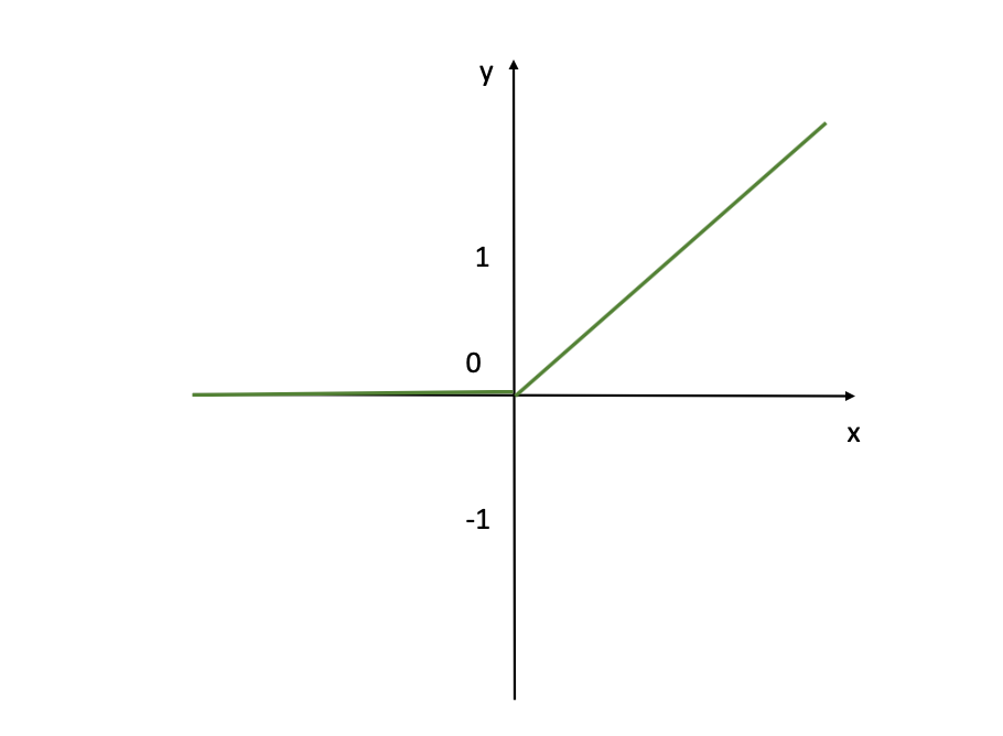
As you may see above from this visualization, the ReLU activation perform doesn’t activate in any respect the enter neurons with unfavourable values (you may see that for the x’s that are unfavourable, corresponding Y-axis worth is 0). While for positiove inputs x, the activation perform returns the precise worth x (Y=X linear line as you see from the determine). But it’s nonetheless default alternative for hidden layers. It is computationally environment friendly and reduces the probability of vanishing gradients throughout coaching, particularly for deep networks.

Leaky ReLU Activation Function

While ReLU doesn’t activate enter neurons with unfavourable values, the Leaky ReLU does account for these unfavourable enter values. It learns from it although with a decrease fee equal to 0.01.

This activation perform might be expressed as follows:

$$

f(z) =
start{circumstances}
0.01z & textual content{if } z < 0
z & textual content{if } z geq 0
finish{circumstances}
$$

So, the Leaky ReLU permits for a small or non-zero gradient when the enter worth is saturated and never lively.

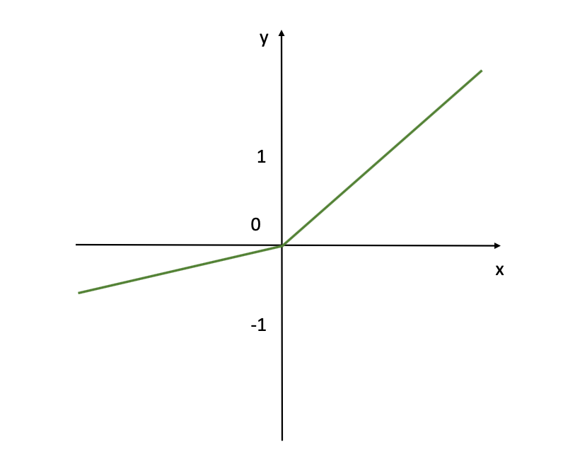
This visualization reveals the Leaky ReLU activation perform generally used neural networks particularly for the hidden layers and the place unfavourable activations is appropriate. Unlike the usual ReLU, which supplies an output of zero for any unfavourable enter, Leaky ReLU permits a small, non-zero output for unfavourable inputs.

Like ReLU, Leaky ReLU can also be default alternative for hidden layers. It is computationally environment friendly and reduces the probability of vanishing gradients throughout coaching, particularly for deep networks with a number of hidden layers.We will speak extra on these and former activations capabilities when discussing the Vanishing Gradient Problem, and if you’d like bit extra particulars and the idea to be defined in tutorial – try the assets beneath.

Hyperbolic Tangent (Tanh) Activation Function

Hyperbolic Tangent activation perform is commonly referred to easily because the Tanh perform. It’s similar to the Sigmoid activation perform. It even has the identical S-shape illustration.

This perform takes any actual worth as enter worth and outputs a worth within the vary -1 to 1. This activation perform might be expressed as follows:

$$

f(z) = tanh(z) = frac{e^z – e^{-z}}{e^z + e^{-z}}
$$

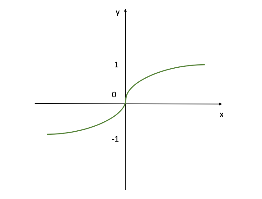
The determine reveals the tanh (hyperbolic tangent) activation perform. So, this perform outputs values starting from -1 to 1, offering a normalized output that may assist with the convergence of neural networks throughout coaching. It’s much like the sigmoid perform however it’s adjusted to permit for unfavourable outputs, which might be helpful for sure varieties of neural networks the place the imply of the outputs must be centered round zero.

Note – if you wish to get extra particulars about these activation capabilities, try this tutorial the place I cowl this idea in additional element at “What is an Activation Function” and “How to Solve the Vanishing Gradient Problem”.

Again, the present default or hottest activation perform for hidden layers is the Rectifier Linear Unit (ReLU) or Softmax perform, primarily for accuracy/efficiency causes. For the output layer, the activation perform is especially chosen based mostly on the format of the predictions (likelihood, scaler, and so forth).

Chapter 3: How to Train Neural Networks

Training neural networks is a scientific course of that entails two principal processes, executed repeatedly, named ahead and backward passes.

First the information goes via the Forward Pass till the output. Then it’s adopted by a backward cross. The thought behind this course of is to undergo the community on a number of events to regulate the weights and reduce the loss or price capabilities.

To get a greater understanding, we’ll look right into a easy Neural Network the place we now have 3 enter indicators, and only a single hidden layer that has 4 hidden models. This might be visualized as follows:

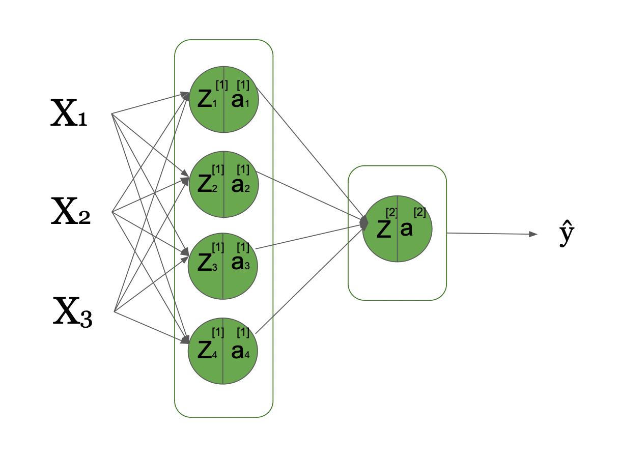
Here you may see that we now have 3 enter indicators in our enter layer, 1 hidden layer with 4 hidden models, and 1 output layer. This is a computational graph visualizing this fundamental neural community and the way the knowledge flows from the left, preliminary inputs to the precise, all the way in which right down to the anticipated Y^ (Y hat), after going via a number of transformations.  

Now, let’s look into this determine that showcases the excessive stage thought of circulation of knowledge.

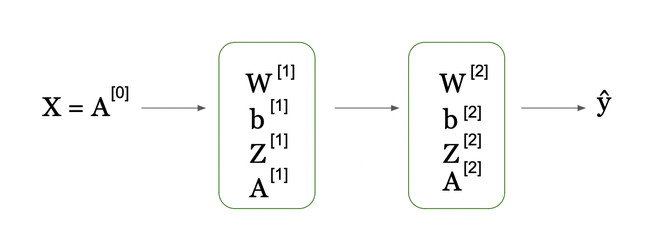
• We go from enter X (which we outline by A[0] because the preliminary activations)
• Then per step (listed by [1]) we take the weights matrix (W[1] and bias vector b[1]) and compute the Z scores (Z[1])
• Then we apply the activation perform to get activation scores (A[1]) at stage [1]. This occurs at time step 1, which is in our instance hidden layer 1.

As we get a single layer, the following step is the output layer, the place the knowledge from the earlier layer (A[1]) is used to compute the brand new Z[2] scores by combining the enter A[1] from the earlier layer and with W[2] / b[2] from this layer. We then apply one other activation layer (our output layer activation perform) on the simply computed Z[2] to compute the A[2].

As the A[2] is within the output layer, this provides us our prediction, Y_hat. This is the Forward Pass or Forward Propagation.

Next you may see within the second a part of the determine, we go from Y_hat to all these phrases which might be form of the identical as in ahead cross however with one essential distinction: all of them have “d” in entrance of them, which refers back to the “spinoff”.

So, after the Y_hat is produced, we get our predictions, and the community is ready to evaluate the Y_hat (predicted values of response variable y, in our instance home value) to the true home costs Y and acquire the Loss perform.

If you need to be taught extra about Loss Functions, try right here or this tutorial.

Then, the community computes the spinoff of loss perform with regard to activations A and Z rating (dA and dZ). Then it makes use of these to compute the gradients/derivatives with regard to the weights W and biases b (dW and db).

This additionally occurs per layer and in a sequential manner, however as you may see from the arrow within the determine above, this time it occurs backwards from proper to left not like in ahead propagation.

This can also be why we refer this course of as backpropagation. The gradients of layer 2 contribute to the calculation of the gradients in layer 1, as you too can see from the graph.

Forward Pass

Forward propagation is the method of feeding enter information via a neural community to generate an output. We will outline the enter information by X which incorporates 3 options X1, X2, X3 which might be described mathematically as follows:

$$
z^i = omega^T x^i + b
$$
$$
Downarrow
$$
$$
hat{y}^i = a^i = sigma(z^i)
$$
$$
Downarrow
$$
$$
l(a^i, y^i)
$$

Where in these equations we’re transferring from enter x_i in our easy neural community, to the calculation of loss.

Let’s unpack them:

Step 1: Each neuron in subsequent layers calculates a weighted sum of its inputs (x^i) plus a bias time period b. We name this a rating z^i. The inputs are the outputs from the earlier layer’s neurons, and the weights in addition to the bias are the parameters that neural community is aiming to be taught and estimate.

Step 2: Then utilizing an activation perform, which we denote by the Greek letter delta, the community transforms the Z scores to a brand new worth which we outline by a^i. Note that the activation worth on the preliminary cross after we are on the preliminary layer within the community (layer 0) is the same as x^i. This is then the anticipated worth in that particular cross.

To be extra correct, let’s make our notation a bit extra difficult. We’ll outline every rating within the first hidden layer, layer [1], per unit (as we now have 4 models on this hidden unit) and generalize this per hidden unit i:

$$
z^{[1]}_i = (omega^{[1]}_i)^T x + (b^{[1]}_i)^T quad textual content{for } i = {1, 2, 3, 4}
$$
$$
a^{[1]}_i = sigma left( z^{[1]}_i proper)
$$

Let’s now rewrite this utilizing Linear Algebra and particularly matrix and vector operations:

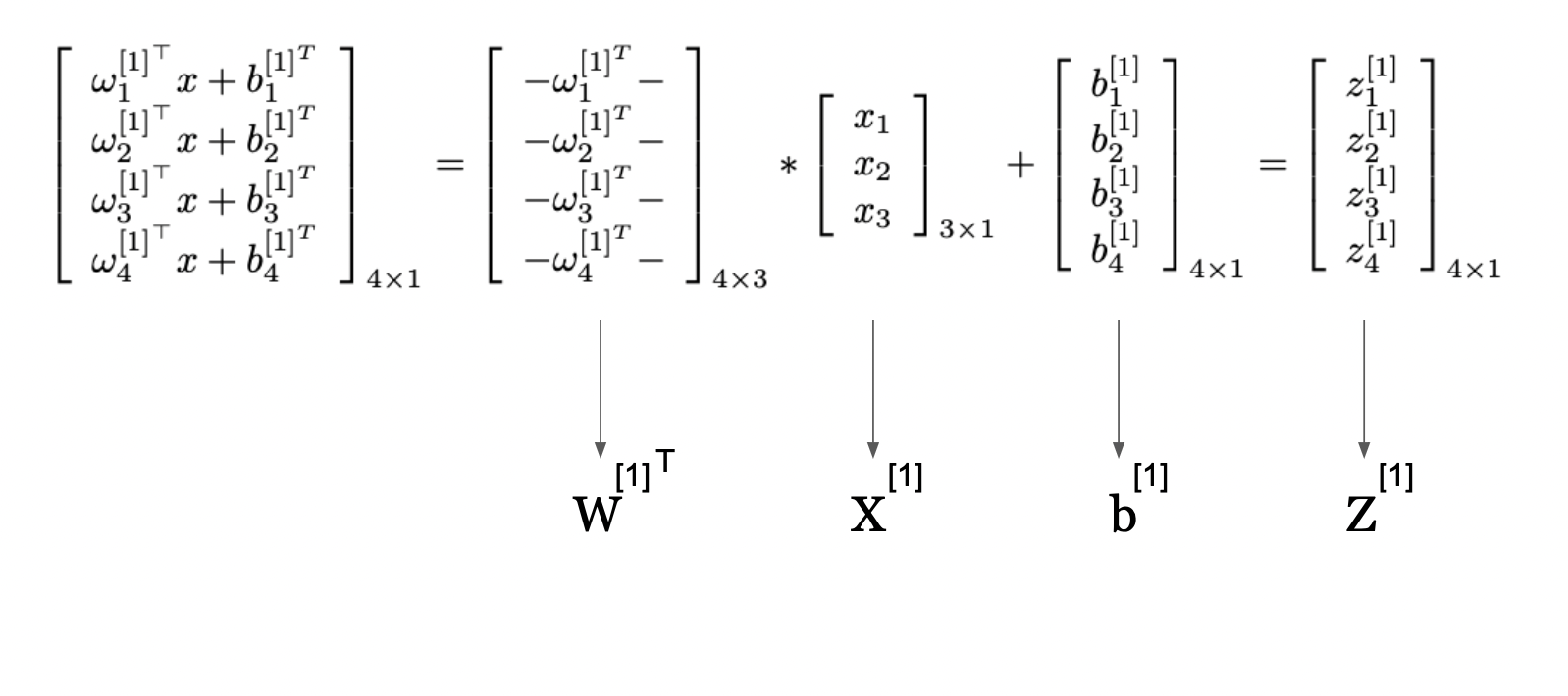
$$
Z^{[1]} = W^{[1]T} X^{[1]} + b^{[1]}
$$

This picture presents a technique to signify the computations in a neural community layer utilizing matrix operations from Linear Algebra. It reveals how particular person computations for every neuron in a layer might be compactly expressed and carried out concurrently via utilizing matrix multiplication and summation.

The matrix labeled  W^[1] incorporates the weights utilized to the inputs for every neuron within the first hidden layer. The vector X[1] is the enter to the layer. By multiplying the load matrix with the enter vector after which including the bias vector b[1], we get the vector Z[1], which we refered as Z-score beforehand too and represents the weighted sum of inputs plus the bias for every neuron.

This compact kind permits us to make use of environment friendly linear algebra routines to compute the outputs of all neurons within the layer directly.

This strategy is key in neural networks because it allows the processing of inputs via a number of layers effectively, permitting neural networks to scale to giant numbers of neurons and complicated architectures.

So, right here we go from unit stage to representing the transformations in our easy neural networks by utilizing Matrix multiplication and summations from Linear Algebra.  

First Layer Activation

$$
Z^{[1]} = W^{[1]T} X^{[1]} + b^{[1]} quad X^{[1]} = A^{[0]}

A^{[1]} = g^{[1]}(Z^{[1]})
$$

Now, let’s look into this equation that showcases the excessive stage thought of circulation of knowledge after we go from enter X[1] (which we outline by A[0] because the preliminary activations) then per step (listed by [1]) we take the weights matrix (W[1] and bias vector b[1]) and compute the Z scores (Z[1]). Then we apply activation perform of layer 1, g[1] to get activation scores (A[1]) at stage [1]. This occurs at time step 1, which is in our instance hidden layer 1.

Second (Output) Layer Activation

$$

Z^{[2]} = W^{[2]T} A^{[1]} + b^{[2]}

A^{[2]} = g^{[2]}(Z^{[2]})

$$

As we get a single layer, subsequent step is the output layer, the place the knowledge from the earlier layer (A[1]) is used to compute the brand new Z[2] scores by combining the enter A[1] from earlier layer and with W[2] / b[2] from this layer. We then apply one other activation perform g[2] (our output layer activation perform) on simply computed Z[2] to compute the A[2].

After the activation perform has been utilized, it will probably then be fed into the following layer of the community if there’s one, or on to the output layer if it is a single hidden layer community. As in our case, layer 2 is our output layer, we’re able to go to Y_hat, our predictions.

This picture reveals a technique to signify the computations in a neural community layer utilizing matrix operations. It reveals how particular person computations for every neuron in a layer of neural community might be compactly expressed, carried out concurrently via matrix multiplication and addition.

Here, the matrix labeled W[1]  incorporates the weights utilized to the inputs for every neuron within the first hidden layer. The vector X[1] is the enter to this layer. By multiplying the load matrix by the enter vector after which including the bias vector b[1], we get  vector Z[1], which represents the weighted sum of inputs plus the bias for every neuron.

This compact kind permits us to make use of environment friendly linear algebra routines to compute the outputs of all neurons within the layer directly. The ensuing vector Z[1] is then handed via an activation perform (not proven on this a part of the picture), which performs a non-linear transformation on every aspect, ensuing within the ultimate output of the layer.

This strategy is key in neural networks because it allows the processing of inputs via a number of layers effectively, permitting neural networks to scale to giant numbers of neurons and complicated architectures.

Computing the Loss Function

As the A[2] is within the output layer, this provides us our prediction, Y_hat. After the Y_hat is produced, we received our predictions, and the community is ready to evaluate the Y_hat (predicted values of response variable y, in our instance home value) to the true home costs Y, and acquire the Loss perform J. The whole loss might be calculated as follows:

$$J = – (Y log(A^{[2]}) + (1 – Y) log(1 – A^{[2]}))$$

the place log() is the logarithm used to compute this loss perform.

Backward Pass

Backpropagation is a vital a part of the coaching technique of a neural community. Combined with optimization algorithms like Gradient Descent (GD), Stochastic Gradient Descent (SGD), or Adam, they carry out the Backward Pass.

Backpropogation is an environment friendly algorithm for computing the gradient of the fee (loss) perform (J) with respect to every parameter (weight & bias) within the community.

So, to be clear, backpropagation is the precise technique of calculating the gradients within the mannequin, after which Gradient Descent is the algorithm that takes the gradients as enter and updates the parameters.

When we compute the gradients and use them to replace the parameters within the mannequin, this helps us replace the parameters and direct them in direction of extra appropriate course in direction of discovering the worldwide optimum to attenuate. This helps additional reduce the loss perform  and  enhance prediction accuracy of the mannequin.

In every cross, after ahead propagation is accomplished, the gradients needs to be obtained. Then we use them to acquire the mannequin parameters, akin to the load and the bias parameters.

Let’s take a look at an instance of the gradient calculations for backpropagation in a neural community that we noticed in Forward Propagation with a single hidden layer and 4 hidden models.

Backpropagation all the time begins from the tip, so let’s visualize it that will help you perceive this course of higher:

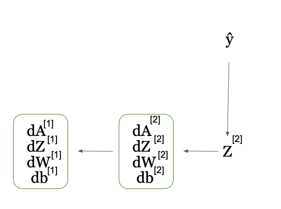
In this determine, the community computes the spinoff of the loss perform with regard to activations A and Z rating (dA and dZ). It then makes use of these to compute the gradients/derivatives with regard to weights W and biases b (dW and db). This additionally occurs per layer and in sequential manner, however as you may see from the arrow within the determine, this time it occurs backwards from proper to left not like in ahead propagation.

This can also be why we refer this course of as backpropagation. The gradients of layer 2 contribute to the calculation of the gradients in layer 1 as you too can see from the graph.

So, the concept is that we calculate the gradients with respect to the activation (dA[2]), then with respect to the pre-activation (dZ[2]), and with respect the weights (dW[2]) and bias (db[2]) of the output layer, assuming we now have a price perform J after we now have computed the Y^. Make certain to all the time cache the Z[i] as they’re wanted on this course of.

Mathematically, the gradients might be calculated utilizing the widespread differentiation guidelines together with acquiring the spinoff of the logarithm, and utilizing Sum Rule and Chain Rules. The first gradient dA[2] might be expressed as follows:

$$
start{align*}
frac{dmathcal{L}}{dA^{[2]}} &= frac{dmathcal{J}}{dA^{[2]}}
downarrow
dA^{[2]} &= left( -frac{d(Ylog(A^{[2]}))}{dA^{[2]}} – frac{d((1 – Y)log(1 – A^{[2]}))}{dA^{[2]}} proper)
downarrow
dA^{[2]} &= -frac{Y}{A^{[2]}} + frac{(1 – Y)}{(1 – A^{[2]})}
finish{align*}
$$

The subsequent gradient we have to compute is the gradient of the fee perform with respect to Z[2], that’s dZ[2].

We know the next:

$$
A^{[2]} = sigma(Z^{[2]})
$$
$$

frac{dJ}{dA^{[2]}} = frac{dA^{[2]}}{dZ^{[2]}}
$$
$$

frac{dA^{[2]}}{dZ^{[2]}} = sigma'(Z^{[2]})
$$

So, A[2] = σ(Z[2]), we will then use these derivatives of the sigmoid perform σ'(Z[2]) = σ(Z[2]) * (1 – σ(Z[2])). This might be derived mathematically as follows:

$$
start{align*}
frac{dZ^{[2]}}{dJ} &= frac{dJ}{dZ^{[2]}} \
downarrow
frac{dZ^{[2]}}{dJ} &= frac{dJ}{dA^{[2]}} cdot frac{dA^{[2]}}{dZ^{[2]}} quad textual content{utilizing chain rule} \
downarrow
frac{dZ^{[2]}}{dJ} &= dA^{[2]} cdot sigma'(Z^{[2]}) \
downarrow
frac{dZ^{[2]}}{dJ} &= dA^{[2]} cdot A^{[2]} cdot (1 – A^{[2]})
finish{align*}
$$
$$
start{align*}
sigma(Z^{[2]}) &= frac{1}{1 – e^{Z^{[2]}}} = (1 – e^{-Z^{[2]}})^{-1}
downarrow
sigma'(Z^{[2]}) &= frac{dsigma(Z^{[2]})}{dZ^{[2]}}
downarrow
sigma'(Z^{[2]}) &= -frac{-1}{(1 – e^{Z^{[2]}})^2} cdot (-1) cdot e^{Z^{[2]}}
downarrow
sigma'(Z^{[2]}) &= frac{1}{1 – e^{Z^{[2]}}} cdot frac{e^{Z^{[2]}}}{1 – e^{Z^{[2]}}}
downarrow
sigma'(Z^{[2]}) &= sigma(Z^{[2]}) cdot (1 – sigma(Z^{[2]})) = A^{[2]} cdot (1 – A^{[2]})
finish{align*}
$$

Now after we know the how and the why behind the calculation of the gradient with regard to the Z rating, we will calculate the gradient with regard to the load W. This is essential for updating the load parameter worth (for instance, course).

$$
start{align*}
Z^{[2]} &= W^{[2]T} cdot A^{[1]} + b^{[2]}
downarrow
frac{db^{[2]}}{dZ^{[2]}} &= frac{dJ}{dZ^{[2]}} cdot frac{dZ^{[2]}}{db^{[2]}} quad textual content{utilizing chain rule}
downarrow
db^{[2]} &= dZ^{[2]} cdot 1 + 0 quad textual content{utilizing fixed rule}
downarrow
db^{[2]} &= dZ^{[2]}
finish{align*}
$$

Now on this step, the one factor remaining is to calculate the gradient with regard to the bias, our second parameter b, within the hidden layer, layer 2.

$$
Z^{[2]} = W^{[2]T} cdot A^{[1]} + b^{[2]}

frac{db^{[2]}}{dJ} = frac{dJ}{dZ^{[2]}} cdot frac{dZ^{[2]}}{db^{[2]}} quad textual content{utilizing chain rule}

db^{[2]} = dZ^{[2]} cdot 1 + 0 quad textual content{utilizing fixed rule}

db^{[2]} = dZ^{[2]}
$$

Since b[2] is a bias time period, its spinoff is solely the sum of the gradients dZ[2] throughout all of the coaching examples (which, in a vectorized implementation, is commonly executed by summing dZ[2] throughout the m observations).

Once backpropogation is completed, subsequent step is to make use of these gradients as enter for optimization algorithm like GD, SGD, or others to learn the way the parameters needs to be up to date.

So, we’re lastly able to replace the Weight and Bias parameters of the mannequin on this cross.

Here is an instance utilizing the GD algorithm:

$$
W^{[2]} = W^{[2]} – eta cdot dW^{[2]}
$$

$$
b^{[2]} = b^{[2]} – eta cdot db^{[2]}
$$

Here the η represents the educational parameter assuming the straightforward GD optimization’s algorithm (extra on the optimization algorithms in later chapters).

In the following part, we’ll go into extra element about how you should use numerous optimization algorithms to coach Deep Learning fashions.

Chapter 4: Optimization Algorithms in AI

Once the gradient is computed through backpropagation, the following step is to make use of an optimization algorithm to regulate the weights to attenuate the fee perform.

To be clear, the optimization algorithm takes as enter the calculated gradients and makes use of this to replace mannequin parameters.

These are the preferred optimization algorithms used when coaching Neural Networks:

• Gradient Descent (GD)
• Stochastic Gradient Descent (SGD)
• SGD with Momentum
• RMSProp
• Adam Optimizer

Knowing the basics of the Deep Learning fashions and studying methods to practice these fashions is unquestionably an enormous a part of Deep Learning. If you’ve got learn thus far and the mathematics hasn’t made you drained, congratulations! You have grasped some difficult subjects. But that’s solely a part of the job.

In order to make use of your Deep Learning mannequin to unravel precise issues, you may must optimize it after you’ve got established its baseline. That is, it’s essential to optimize the set of parameters in your Machine Learning mannequin to search out the set of optimum parameters that lead to the most effective performing mannequin (all issues being equal).

So, to optimize or to tune your Machine Learning mannequin, it’s essential to carry out hyperparameter optimization. By discovering the optimum mixture of hyperparameter values, we will lower the errors the mannequin produces and construct probably the most correct neural community.

A mannequin’s hyperparameter is a continuing within the mannequin. It’s exterior to the mannequin, and its worth can’t be estimated from information (however slightly needs to be specified upfront earlier than the mannequin is educated). For occasion, weights and bias parameters in neural community are parameters we need to optimize.

NOTE: As optimization algorithms are used throughout all neural networks, I assumed it will likely be helpful to supply you the Python code which you’ll implement to carry out neural community optimization manually.

Just remember that this isn’t what you’ll do in follow, as there are libraries for this function. Still, seeing the Python code will provide help to to grasp the precise workings of those algorithms like GD, SGD, SGD with Momentum, Adam, AdamW a lot better.

I’ll present you the formulation, explanations, in addition to the Python code so you may see that’s the Python code behind the precise capabilities of the libraries that implement these optimization algorithms.

Gradient Descent (GD)

The Batch Gradient Descent algorithm (typically simply known as Gradient Descent or GD), computes the gradient of the Loss Function J(θ) with respect to the goal parameter utilizing your complete coaching information.

We do that by first predicting the values for all observations in every iteration, and evaluating them to the given worth within the coaching information.

These two values are used to calculate the prediction error time period per commentary which is then used to replace the mannequin parameters. This course of continues till the mannequin converges.

The gradient or the primary order spinoff of the loss perform might be expressed as follows:

$$nabla_{theta} J(theta)$$

Then, this gradient is used to replace the earlier iterations’ worth of the goal parameter. That is:

$$
theta = theta – eta cdot nabla_{theta} J(theta)
$$

In this equation:

• θ represents the parameter(s) or weight(s) of a mannequin that you’re making an attempt to optimize. In many contexts, particularly in neural networks, θ could be a vector containing many particular person weights.
• η is the educational fee. It’s a hyperparameter that dictates the step dimension at every iteration whereas transferring in direction of a minimal of the fee perform. A smaller studying fee may make the optimization extra exact, however might additionally decelerate the convergence course of. A bigger studying fee may velocity up convergence, however dangers overshooting the minimal. This might be [0,1] however is is often a quantity between (0.001 and 0.04)
• ∇J(θ) is the gradient of the fee perform J with respect to the parameter θ. It signifies the course and magnitude of the steepest enhance of J. By subtracting this from the present parameter worth (multiplied by the educational fee), we regulate θ within the course of the steepest lower of J.

In phrases of Neural Networks, within the earlier part we noticed the utilization of this straightforward optimisation method.

There are two main disadvantages to GD which make this optimization method not so in style, particularly when coping with giant and complicated datasets.

Since in every iteration your complete coaching information needs to be used and saved, the computation time might be very giant leading to extremely sluggish course of. On high of that, storing that giant quantity of information leads to reminiscence points, making GD computationally heavy and sluggish.

You can be taught extra on this Gradient Descent Interview Tutorial.

Gradient Descent in Python

Let’s take a look at an instance of methods to use Gradient Descent in Python:

def update_parameters_with_gd(parameters, grads, learning_rate):
    """
    Update parameters utilizing a easy gradient descent replace rule.
    
    Arguments:
    parameters -- python dictionary containing your parameters 
                  (e.g., {"W1": W1, "b1": b1, "W2": W2, "b2": b2, ..., "WL": WL, "bL": bL})
    grads -- python dictionary containing your gradients to replace every parameters 
             (e.g., {"dW1": dW1, "db1": db1, "dW2": dW2, "db2": db2, ..., "dWL": dWL, "dbL": dbL})
    learning_rate -- the educational fee, scalar.
    
    Returns:
    parameters -- python dictionary containing your up to date parameters 
    """

    L = len(parameters) // 2 # variety of layers within the neural networks

    # Update rule for every parameter
    for l in vary(L):
        parameters["W" + str(l+1)] -= learning_rate * grads["dW" + str(l+1)]
        parameters["b" + str(l+1)] -= learning_rate * grads["db" + str(l+1)]
        
    return parameters

This is a Python code snippet implementing gradient descent (GD) algorithm for updating parameters in a neural community which take these three arguments:

1. parameters: dictionary containing present parameters of the neural community (for instance, weights and biases for every layer of neural community)
2. grads: dictionary containing gradients of the parameters, calculated throughout backpropagation
3. learning_rate: scalar worth representing the educational fee, which controls the step dimension of the parameter updates.

This code iterates via the layers of the neural community and updates the weights (W) and biases (b) for every layer utilizing the next replace rule for every parameter:

After looping via all of the layers in neural community, it returns the up to date parameters. This course of helps the neural community to be taught and regulate its parameters to attenuate the loss throughout coaching, in the end bettering its efficiency and leading to extremely correct predictions.

Stochastic Gradient Descent (SGD)

The Stochastic Gradient Descent (SGD) technique, also referred to as Incremental Gradient Descent, is an iterative strategy for fixing optimisation issues with a differential goal perform, precisely like GD.

But not like GD, SGD doesn’t use your complete batch of coaching information to replace the parameter worth in every iteration. The SGD technique is sometimes called the stochastic approximation of the gradient descent. It goals to search out the intense or zero factors of the stochastic mannequin containing parameters that can’t be immediately estimated.

SGD minimises this price perform by sweeping via information within the coaching dataset and updating the values of the parameters in each iteration.

In SGD, all mannequin parameters are improved in every iteration step with just one coaching pattern or a mini-batch. So, as a substitute of going via all coaching samples directly to change mannequin parameters, the SGD algorithm improves parameters by a single and randomly sampled coaching set (therefore the title Stochastic, which suggests “involoving probability or likelihood”).

It adjusts the parameters in the other way of the gradient by a step proportional to the educational fee. The replace at time step t might be given by the next system:

$$
theta_{t+1} = theta_t – eta nabla_{theta} J(theta_t)
$$

In this equation:

• θ represents the parameter(s) or weight(s) of a mannequin that you’re making an attempt to optimize. In many contexts, particularly in neural networks, θ could be a vector containing many particular person weights.
• η is the educational fee. It’s a hyperparameter that dictates the step dimension at every iteration whereas transferring in direction of a minimal of the fee perform. A smaller studying fee may make the optimization extra exact however might additionally decelerate the convergence course of. A bigger studying fee may velocity up convergence however dangers overshooting the minimal.
• ∇J(θt) is the gradient of the fee perform J with respect to the parameter θ for a given enter x(i) and its corresponding goal output y(i) at step t. It signifies the course and magnitude of the steepest enhance of J. By subtracting this from the present parameter worth (multiplied by the educational fee), we regulate θ within the course of the steepest lower of J.
• x(i) represents the ith enter information pattern out of your dataset.
• y(i) is the true goal output for the ithenter information pattern.

In the context of Stochastic Gradient Descent (SGD), the replace rule applies to particular person information samples x(i) and y(i) slightly than your complete dataset, which might be the case for batch Gradient Descent.

This single step improves the velocity of the method of discovering the worldwide minima of the optimization downside and that is what differentiates SGD from GD. So, SGD persistently adjusts the parameters with an try to maneuver within the course of the worldwide minimal of the target perform.

In SGD, all mannequin parameters are improved in every iteration step with just one coaching pattern. So, as a substitute of going via all coaching samples directly to change mannequin parameters, SGD improves parameters by a single coaching pattern.

Though SGD addresses the sluggish computation time situation of GD, as a result of it scales nicely with each huge information and with a dimension of the mannequin, it is named a “unhealthy optimizer” as a result of it’s liable to discovering a neighborhood optimum as a substitute of a world optimum.

SGD might be noisy as a result of this stochastic nature of it, as it’s utilizing gradients calculated from solely a subset of the information (a mini-batch or single level). This can result in variance within the parameter updates.

For extra particulars on SGD, you may try this tutorial.

Example of SGD in Python

Now let’s have a look at methods to implement it in Python:

def update_parameters_with_sgd(parameters, grads, learning_rate):
    """
    Update parameters utilizing SGD
    
    Input Arguments:
    parameters -- dictionary containing your parameters (e.g., weights, biases)
    grads -- dictionary containing gradients to replace every parameters
    learning_rate -- the educational fee, scalar.
    
    Output:
    parameters -- dictionary containing your up to date parameters
    """
    
    for key in parameters:
        # Update rule for every parameter
        parameters[key] = parameters[key] - learning_rate * grads['d' + key]
        
    return parameters

Here’s what is going on on on this code:

• parameters is a dictionary that holds the weights and biases of your community (for instance, parameters['W1'], parameters['b1'], and so forth)
• grads holds the gradients of the weights and biases (for instance, grads['dW1'], grads['db1'], and so forth).
• The perform initialize_velocity() is used to create the speed dictionary earlier than you begin coaching the community with momentum.
• The update_parameters_with_momentum() perform then makes use of this velocity along with the gradients to replace the parameters.

SGD with Momentum

When the error perform is complicated and non-convex, as a substitute of discovering the worldwide optimum, the SGD algorithm mistakenly strikes within the course of quite a few native minima.

In order to handle this situation and additional enhance the SGD algorithm, numerous strategies have been launched. One in style manner of escaping a neighborhood minimal and transferring in the precise course of a world minimal is SGD with Momentum.

The objective of the SGD technique with momentum is to speed up gradient vectors within the course of the worldwide minimal, leading to quicker convergence.

The thought behind the momentum is that the mannequin parameters are realized by utilizing the instructions and values of earlier parameter changes. Also, the adjustment values are calculated in such a manner that more moderen changes are weighted heavier (they get bigger weights) in comparison with the very early changes (they get smaller weights).

Basically, SGD with momentum is designed to speed up the convergence of SGD and to scale back its oscillations. So, it introduces a velocity time period, which is a fraction of the earlier replace. This precise step helps the optimizer construct up velocity in instructions with persistent, constant gradients, and dampens updates in fluctuating instructions.

The replace guidelines for momentum are as follows, the place you first should compute the gradient (as with plain SGD) after which replace velocity and the parameter theta.

$$
v_{t+1} = gamma v_t + eta nabla_{theta} J(theta_t)
$$

$$
theta_{t+1} = theta_t – v_{t+1}
$$

The momentum γ which is usually a worth between 0.5 & 0.9, determines how a lot of previous gradients can be retained and used within the replace.

The purpose for this distinction is that with the SGD technique we don’t decide the precise spinoff of the loss perform, however we estimate it on a small batch. Since the gradient is noisy, it’s possible that it’ll not all the time transfer within the optimum course.

The momentum helps then to estimate these derivatives extra precisely, leading to higher course decisions when transferring in direction of the worldwide minimal.

Another purpose for the distinction within the efficiency of classical SGD and SGD with momentum lies within the space referred as Pathological Curvature, additionally referred to as the ravine space.

Pathological Curvature or Ravine Area might be represented by the next graph. The orange line represents the trail taken by the strategy based mostly on the gradient whereas the darkish blue line represents the best path in in direction of the course of ending the worldwide optimum.

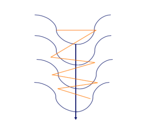
To visualise the distinction between the SGD and SGD Momentum, let’s take a look at the next determine:

On the left hand-side is the SGD technique with out Momentum. On the precise hand-side is the SGD with Momentum. The orange sample represents the trail of the gradient in a search of the worldwide minimal. As you may see, within the left determine we now have extra of those occiliations in comparison with the precise one, and that is the influence of Momentum, the place we speed up the coaching and the algorithm then make much less of this actions.

The thought behind the momentum is that the mannequin parameters are realized by utilizing the instructions and values of earlier parameter changes. Also, the adjustment values are calculated in such a manner that more moderen changes are weighted heavier (they get bigger weights) in comparison with the very early changes (they get smaller weights).

Example of SGD with Momentum in Python

Let’s see what this appears to be like like in code:

def initialize_velocity(parameters):
    """
    Initializes the speed as a python dictionary with:
                - keys: "dW1", "db1", ..., "dWL", "dbL"
                - values: numpy arrays of zeros of the identical form because the corresponding gradients/parameters.
    """
    L = len(parameters) // 2 # variety of layers within the neural networks
    v = {}
    
    for l in vary(L):
        v["dW" + str(l+1)] = np.zeros_like(parameters["W" + str(l+1)])
        v["db" + str(l+1)] = np.zeros_like(parameters["b" + str(l+1)])
        
    return v

def update_parameters_with_momentum(parameters, grads, v, beta, learning_rate):
    """
    Update parameters utilizing Momentum
    
    Arguments:
    parameters -- python dictionary containing your parameters
    grads -- python dictionary containing your gradients for every parameters
    v -- python dictionary containing the present velocity
    beta -- the momentum hyperparameter, scalar
    learning_rate -- the educational fee, scalar
    
    Returns:
    parameters -- python dictionary containing your up to date parameters 
    v -- python dictionary containing your up to date velocities
    """
    
    L = len(parameters) // 2 # variety of layers within the neural networks
    
    # Momentum replace for every parameter
    for l in vary(L):
        # compute velocities
        v["dW" + str(l+1)] = beta * v["dW" + str(l+1)] + (1 - beta) * grads["dW" + str(l+1)]
        v["db" + str(l+1)] = beta * v["db" + str(l+1)] + (1 - beta) * grads["db" + str(l+1)]
        # replace parameters
        parameters["W" + str(l+1)] = parameters["W" + str(l+1)] - learning_rate * v["dW" + str(l+1)]
        parameters["b" + str(l+1)] = parameters["b" + str(l+1)] - learning_rate * v["db" + str(l+1)]
        
    return parameters, v

In this code we now have two capabilities for implementing the momentum-based gradient descent algorithm (SGD with momentum):

1. initialize_velocity(parameters): This perform initializes the speed for every parameter within the neural community. It takes the present parameters as enter and returns a dictionary (v) with keys for gradients (“dW1”, “db1”, …, “dWL”, “dbL”) and initializes the corresponding values as numpy arrays full of zeros.
2. update_parameters_with_momentum(parameters, grads, v, beta, learning_rate): This perform updates the parameters utilizing Momentum optimization method. It takes the next arguments:
3. parameters: dictionary containing  present parameters of the neural community.
4. grads: dictionary containing the gradients of the parameters.
5. v: dictionary containing the present velocities of the parameters (initialized utilizing the initialize_velocity (perform).
6. beta: momentum hyperparameter, a scalar that controls the affect of previous gradients on the updates.
7. learning_rate: studying fee, a scalar controlling the step dimension of the parameter updates.

Inside the perform, it iterates via the layers of the neural community and performs the next steps for every parameter:

• Computes new velocity utilizing the momentum system.
• Updates parameter utilizing new velocity and studying fee.
• Finally, it returns the up to date parameters and velocities.

RMSProp

Root Mean Square Propagation, generally referred to as RMSprop, is an optimization technique with an adaptive studying fee. It was proposed by Geoff Hinton in his Coursera class.

RMSprop adjusts studying fee for every parameter by dividing the educational fee for a weight by a working common of magnitudes of current gradients for that weight.

RMSprop might be outlined mathematically as follows:

$$
v_t = beta v_{t-1} + (1 – beta) g_t^2
$$

$$
theta_{t+1} = theta_t – frac{eta}{sqrt{v_t + epsilon}} cdot g_t
$$

• vt​ is the working common of the squared gradients.
• β is the decay fee that controls the transferring common (often set to 0.9).
• η is the educational fee.
• ϵ is a small scalar used to stop division by zero (often round 10^-8).
• gt​ is the gradient at time step t, and θt​ is parameter vector at time step t.

The algorithm first calculates the working common of the squared gradients (the hessian) for every parameter: v_t at step t.

Then it divides the educational fee eta by the sq. root of this common velocity (element-wise division if the parameters are vectors or matrices). Then it makes use of this in the identical step to replace the parameters.

Example of RMSProp in Python

Here’s an instance of the way it works in Python:

def update_parameters_with_rmsprop(parameters, grads, s, learning_rate, beta, epsilon):
    """
    Update parameters utilizing RMSprop.
    
    Arguments:
    parameters -- python dictionary containing your parameters 
                    (e.g., {"W1": W1, "b1": b1, "W2": W2, "b2": b2})
    grads -- python dictionary containing your gradients to replace every parameters 
                    (e.g., {"dW1": dW1, "db1": db1, "dW2": dW2, "db2": db2})
    s -- python dictionary containing the working common of the squared gradients 
                    (e.g., {"dW1": s_dW1, "db1": s_db1, "dW2": s_dW2, "db2": s_db2})
    learning_rate -- the educational fee, scalar.
    beta -- the momentum hyperparameter, scalar.
    epsilon -- small quantity to keep away from division by zero, scalar.
    
    Returns:
    parameters -- python dictionary containing your up to date parameters 
    s -- python dictionary containing the up to date working common of the squared gradients
    """
    
    L = len(parameters) // 2 # variety of layers within the neural networks

    # Update rule for every parameter
    for l in vary(L):
        # Compute transferring common of the squared gradients
        s["dW" + str(l+1)] = beta * s["dW" + str(l+1)] + (1 - beta) * np.sq.(grads["dW" + str(l+1)])
        s["db" + str(l+1)] = beta * s["db" + str(l+1)] + (1 - beta) * np.sq.(grads["db" + str(l+1)])
        
        # Update parameters
        parameters["W" + str(l+1)] -= learning_rate * grads["dW" + str(l+1)] / (np.sqrt(s["dW" + str(l+1)]) + epsilon)
        parameters["b" + str(l+1)] -= learning_rate * grads["db" + str(l+1)] / (np.sqrt(s["db" + str(l+1)]) + epsilon)

    return parameters, s

This code defines a perform for updating neural community parameters utilizing the RMSprop optimization method. Here’s a abstract of the perform:

• update_parameters_with_rmsprop(parameters, grads, s, learning_rate, beta, epsilon):  perform updates parameters of a neural community utilizing RMSprop.

It takes the next arguments:

• parameters: dictionary containing present parameters of the neural community.
• grads: dictionary containing gradients of the parameters.
• s: dictionary containing working common of squared gradients for every parameter.
• learning_rate: studying fee, a scalar.
• beta: momentum hyperparameter, a scalar.
• epsilon: A small quantity added to stop division by zero, a scalar.

Inside this perform, the code iterates via the layers of the neural community and performs the next steps for every parameter:

• Computes the transferring common of the squared gradients for each weights (W) and biases (b) utilizing the RMSprop system.
• Updates the parameters utilizing the computed transferring averages and the educational fee, with an extra epsilon time period within the denominator to keep away from division by zero.

Finally, the code returns up to date parameters and up to date working common of the squared gradients (s).

RMSprop is an optimization method that adapts the educational fee for every parameter based mostly on the historical past of squared gradients. It helps stabilize and speed up coaching, notably when coping with sparse or noisy gradients.

Adam Optimizer

Another in style method for enhancing the SGD optimization process is the Adaptive Moment Estimation (Adam) launched by Kingma and Ba (2015). Adam mainly combines SGD momentum with RMSProp.

The principal distinction in comparison with the SGD with momentum, which makes use of a single studying fee for all parameter updates, is that the Adam algorithm defines totally different studying charges for various parameters.

The algorithm calculates the person adaptive studying charges for every parameter based mostly on the estimates of the primary two moments of the gradients (first and the second order spinoff of the Loss perform).

So, every parameter has a novel studying fee, which is being up to date utilizing the exponential decaying common of the primary moments (the imply) and second moments (the variance) of the gradients.

Basically, Adam, computes particular person adaptive studying charges for various parameters from estimates of 1st and 2nd moments of gradients.

The replace guidelines for the Adam optimizer might be expressed as follows:

1. Calculate working averages of each the gradients and squared gradients
2. Adjust these working averages for a bias issue
3. Use these working averages to replace the educational fee for every parameter individually

Mathematically, these steps are represented as follows:

$$
m_t = beta_1 m_{t-1} + (1 – beta_1) g_t
$$
$$
v_t = beta_2 v_{t-1} + (1 – beta_2) g_t^2
$$
$$
hat{m}_t = frac{m_t}{1 – beta_1^t}
$$
$$
hat{v}_t = frac{v_t}{1 – beta_2^t}
$$
$$
theta_{t+1} = theta_t – alpha cdot frac{hat{m}_t}{sqrt{hat{v}_t} + epsilon}
$$

• mt​ and vt are estimates of the primary second (the imply) and the second second (the uncentered variance) of the gradients, respectively.
• m_hat and v_hat are bias-corrected variations of those estimates.
• β1​ and β2​ are the exponential decay charges for these second estimates (often set to 0.9 & 0.999, respectively).
• α is the educational fee.
• ϵ is a small scalar used to stop division by zero (often round 10^(–8)).

Example of Adam in Python

Here’s an instance of utilizing Adam in Python:

def initialize_adam(parameters) :
    """
    Initializes v and s as two python dictionaries with:
                - keys: "dW1", "db1", ..., "dWL", "dbL"
                - values: numpy arrays of zeros of the identical form because the corresponding gradients/parameters.
    """
    
    L = len(parameters) // 2 # variety of layers within the neural networks
    v = {}
    s = {}
    
    for l in vary(L):
        v["dW" + str(l+1)] = np.zeros_like(parameters["W" + str(l+1)])
        v["db" + str(l+1)] = np.zeros_like(parameters["b" + str(l+1)])
        s["dW" + str(l+1)] = np.zeros_like(parameters["W" + str(l+1)])
        s["db" + str(l+1)] = np.zeros_like(parameters["b" + str(l+1)])
    
    return v, s

def update_parameters_with_adam(parameters, grads, v, s, t, learning_rate=0.01,
                                beta1=0.9, beta2=0.999, epsilon=1e-8):
    """
    Update parameters utilizing Adam
    
    Arguments:
    parameters -- python dictionary containing your parameters:
                    parameters['W' + str(l)] = Wl
                    parameters['b' + str(l)] = bl
    grads -- python dictionary containing your gradients for every parameters:
                    grads['dW' + str(l)] = dWl
                    grads['db' + str(l)] = dbl
    v -- Adam variable, transferring common of the primary gradient, python dictionary
    s -- Adam variable, transferring common of the squared gradient, python dictionary
    learning_rate -- the educational fee, scalar.
    beta1 -- Exponential decay hyperparameter for the primary second estimates 
    beta2 -- Exponential decay hyperparameter for the second second estimates 
    epsilon -- hyperparameter stopping division by zero in Adam updates

    Returns:
    parameters -- python dictionary containing your up to date parameters 
    v -- Adam variable, transferring common of the primary gradient, python dictionary
    s -- Adam variable, transferring common of the squared gradient, python dictionary
    """
    
    L = len(parameters) // 2                 # variety of layers within the neural networks
    v_corrected = {}                         # Initializing first second estimate, python dictionary
    s_corrected = {}                         # Initializing second second estimate, python dictionary
    
    # Perform Adam replace on all parameters
    for l in vary(L):
        # Moving common of the gradients.
        v["dW" + str(l+1)] = beta1 * v["dW" + str(l+1)] + (1 - beta1) * grads["dW

In this code we implement Adam algorithm, consisting of two functions:

1. initialize_adam(parameters): This function initializes the Adam optimizer variables v and s as two Python dictionaries. It takes the current parameters as input and returns v and s, both of which are dictionaries with keys for gradients (“dW1”, “db1”, …, “dWL”, “dbL”). The values are numpy arrays filled with zeros and have the same shape as the corresponding gradients/parameters.
2. update_parameters_with_adam(parameters, grads, v, s, t, learning_rate=0.01, beta1=0.9, beta2=0.999, epsilon=1e-8): This function updates the parameters of a neural network using the Adam optimization technique. It takes the following arguments:
3. parameters: A dictionary containing the current parameters of the neural network.
4. grads: A dictionary containing the gradients of the parameters.
5. v: A dictionary representing the moving average of the first gradient moments.
6. s: A dictionary representing the moving average of the squared gradient moments.
7. t: A scalar representing the current time step (used for bias correction).
8. learning_rate: The learning rate, a scalar.
9. beta1: The exponential decay hyperparameter for the first moment estimates.
10. beta2: The exponential decay hyperparameter for the second moment estimates.
11. epsilon: A small number added to prevent division by zero in Adam updates.

Inside this function, code iterates through layers of the neural network and performs Adam updates for each parameter. This includes computing moving averages of gradients and squared gradients, and using these values to update the parameters. It also performs bias correction to adjust the moving averages.

Finally, code returns the updated parameters, v (first moment estimates), and s (second moment estimates).

AdamW

AdamW (the ‘W’ stands for ‘Weight Decay’) is a optimization algorithm which modifies the way weight decay is integrated into the original Adam algorithm. This seemingly small change has significant implications for the training process, particularly in how it manages regularization to prevent overfitting.

This step has a crucial impact in making deep learning model more generalizable, for building models that generalize well to new, unseen data.

In traditional optimizers like SGD, the weight decay directly regularizes the model’s weight parameters. But, in Adam, this process is somewhat conflated with the optimizer’s adaptive learning rates.

AdamW decouples weight decay from the learning rates, reinstating the direct regularization effect seen in SGD. This results in more effective regularization and, often, better performance in training deep neural networks.

If you want to see the actual mathematical representation where I am comparing Adam and AdamW, you can check out this Tutorial on YouTube.

By choosing AdamW, you can enjoy the benefits of adaptive learning rates while maintaining a more robust regularization mechanism.

This optimization algorithm has quickly gained popularity in the machine learning community, particularly among those working on large-scale models and complex datasets where every bit of optimization efficiency counts.

AdamW in Python

import numpy as np

def initialize_adamw(parameters):
    """
    Initializes v, s, and w as three python dictionaries with:
                - keys: "dW1", "db1", ..., "dWL", "dbL"
                - values: numpy arrays of zeros of the same shape as the corresponding gradients/parameters.
    """
    
    L = len(parameters) // 2  # number of layers in the neural network
    v = {}
    s = {}
    w = {}
    
    for l in range(L):
        v["dW" + str(l+1)] = np.zeros_like(parameters["W" + str(l+1)])
        v["db" + str(l+1)] = np.zeros_like(parameters["b" + str(l+1)])
        s["dW" + str(l+1)] = np.zeros_like(parameters["W" + str(l+1)])
        s["db" + str(l+1)] = np.zeros_like(parameters["b" + str(l+1)])
        w["W" + str(l+1)] = np.copy(parameters["W" + str(l+1)])
    
    return v, s, w

def update_parameters_with_adamw(parameters, grads, v, s, w, t, learning_rate=0.01,
                                beta1=0.9, beta2=0.999, epsilon=1e-8, weight_decay=0.01):
    """
    Update parameters utilizing AdamW (Adam with weight decay)
    
    Arguments:
    parameters -- python dictionary containing your parameters:
                    parameters['W' + str(l)] = Wl
                    parameters['b' + str(l)] = bl
    grads -- python dictionary containing your gradients for every parameter:
                    grads['dW' + str(l)] = dWl
                    grads['db' + str(l)] = dbl
    v -- Adam variable, transferring common of the primary gradient, python dictionary
    s -- Adam variable, transferring common of the squared gradient, python dictionary
    w -- Weight parameters for weight decay, python dictionary
    t -- Current time step (used for bias correction), scalar
    learning_rate -- The studying fee, scalar
    beta1 -- Exponential decay hyperparameter for the primary second estimates 
    beta2 -- Exponential decay hyperparameter for the second second estimates 
    epsilon -- Hyperparameter stopping division by zero in Adam updates
    weight_decay -- Weight decay hyperparameter, scalar

    Returns:
    parameters -- python dictionary containing your up to date parameters 
    v -- Adam variable, transferring common of the primary gradient, python dictionary
    s -- Adam variable, transferring common of the squared gradient, python dictionary
    """
    
    L = len(parameters) // 2  # variety of layers within the neural community
    v_corrected = {}          # Initializing first second estimate, python dictionary
    s_corrected = {}          # Initializing second second estimate, python dictionary
    
    # Perform AdamW replace on all parameters
    for l in vary(L):
        # Moving common of the gradients
        v["dW" + str(l+1)] = beta1 * v["dW" + str(l+1)] + (1 - beta1) * grads["dW" + str(l+1)]
        v["db" + str(l+1)] = beta1 * v["db" + str(l+1)] + (1 - beta1) * grads["db" + str(l+1)]
        
        # Moving common of the squared gradients
        s["dW" + str(l+1)] = beta2 * s["dW" + str(l+1)] + (1 - beta2) * np.sq.(grads["dW" + str(l+1)])
        s["db" + str(l+1)] = beta2 * s["db" + str(l+1)] + (1 - beta2) * np.sq.(grads["db" + str(l+1)])
        
        # Bias correction for transferring averages
        v_corrected["dW" + str(l+1)] = v["dW" + str(l+1)] / (1 - np.energy(beta1, t))
        v_corrected["db" + str(l+1)] = v["db" + str(l+1)] / (1 - np.energy(beta1, t))
        s_corrected["dW" + str(l+1)] = s["dW" + str(l+1)] / (1 - np.energy(beta2, t))
        s_corrected["db" + str(l+1)] = s["db" + str(l+1)] / (1 - np.energy(beta2, t))
        
        # Update parameters with weight decay
        parameters["W" + str(l+1)] -= learning_rate * (v_corrected["dW" + str(l+1)] / (np.sqrt(s_corrected["dW" + str(l+1)]) + epsilon) + weight_decay * w["W" + str(l+1)])
        parameters["b" + str(l+1)] -= learning_rate * (v_corrected["db" + str(l+1)] / (np.sqrt(s_corrected["db" + str(l+1)]) + epsilon) + weight_decay * w["W" + str(l+1)])
    
    return parameters, v, s

In this  code  we implement AdamW optimization algorithm, which is an extension of the Adam optimizer with added weight decay regularization. Let’s undergo every a part of the code:

• initialize_adamw(parameters): This perform initializes AdamW optimizer variables. It takes all the present parameters of a neural community as enter and returns three dictionaries: v, s, and w.

Here’s what every of those dictionaries represents:

• v: A dictionary for the transferring common of the primary gradient moments. It has keys like “dW1”, “db1”, …, “dWL”, “dbL”, and the values are initialized as numpy arrays full of zeros of the identical form because the corresponding gradients/parameters.
• s: A dictionary for the transferring common of the squared gradient moments, much like v.
• w: A dictionary for weight parameters used for weight decay. It is initialized with a replica of the present weight parameters.

update_parameters_with_adamw(parameters, grads, v, s, w, t, learning_rate=0.01, beta1=0.9, beta2=0.999, epsilon=1e-8, weight_decay=0.01): This perform performs AdamW as we noticed within the equations, to replace on the neural community parameters. It takes a number of arguments:

• parameters: A dictionary containing the present parameters of the neural community.
• grads: A dictionary containing the gradients of the parameters, calculated throughout backpropagation.
• v: dictionary representing the transferring common of the primary gradient moments.
• s: dictionary representing the transferring common of the squared gradient moments.
• w: dictionary containing weight parameters for weight decay.
• t: scalar representing the present time step (used for bias correction).
• learning_rate: The studying fee, a scalar.
• beta1:  exponential decay hyperparameter for the primary second estimates (usually near 1).
• beta2: exponential decay hyperparameter for the second second estimates (usually near 1).
• epsilon: small quantity added to stop division by zero in Adam updates.
• weight_decay: weight decay hyperparameter, which controls the energy of L2 regularization.

Inside the perform, the next steps are carried out for every parameter:

1. Update v and s utilizing the gradients, much like the usual Adam replace.
2. Perform bias correction on v and s to account for the truth that they’re initialized with zeros and could also be biased in direction of zero.
3. Update parameters with weight decay regularization. Weight decay encourages smaller parameter values by subtracting a fraction of the present weight from the replace.
4. Return the up to date parameters, v, and s.

Chapter 5: Regularization and Generalization

In this chapter, we’ll dive into some essential ideas in Deep Learning, like:

• Overfitting & underfitting in neural networks
• Regularization methods: Dropout, L1/L2 regularization, batch normalization
• Data augmentation & its function in bettering mannequin robustness

Let’s get began.

The Dropout Regularization Technique

Dropout is without doubt one of the hottest regularization methods used to stop overfitting in neural networks. The manner the algorithm works is that it randomly “drops out” (that’s, it units to zero) numerous output options of the layer throughout coaching.

During the coaching course of, after calculating the activations, the algorithm randomly units fraction p (the dropout fee) of the activations to zero. These options are then not getting used throughout the coaching course of in that cross. This dropout fee p is a hyperparameter usually set between 0.2 and 0.5. Note that this drop-out fee is barely used throughout coaching.

For every layer l, for every coaching instance i, and for every neuron/unit j, the dropout might be mathematically represented as follows:

Where:

• rj(l)​ is a random variable that follows Bernoulli distribution, the place the likelihood of not being dropped out (success: 1) is 1−p.
• aj(l)​ is the activation of neuron j in layer l.
• a~j(l)​ is the activation of neuron j after making use of dropout.

During backpropagation within the coaching course of, the gradients are solely handed via the neurons that weren’t dropped out (when there was successful in Bernoulli trial). Remember that this drop-out fee is barely used throughout coaching.

Testing Adjustment: During testing course of, the dropout shouldn’t be utilized. Instead, the activations are scaled down by an element of p to account for the impact of dropout throughout coaching course of. This is critical as a result of throughout coaching, on common, every unit is barely lively with likelihood 1−p.

This ensures that the anticipated sum of the activations is similar throughout coaching and take a look at time.

Dropout successfully creates a “thinned” community with a unique structure for every coaching step. Because the community structure is totally different for every coaching pattern as we randomly flip off a number of the neurons, this may be seen as of coaching a set of networks with shared weights.

During testing, you get the good thing about averaging the consequences of those totally different networks, which tends to scale back overfitting. This is as a result of it introduces beat bias, however extra importantly, it considerably reduces variance when the mannequin is used for prediction. Here’s why:

Introducing Bias

By dropping out totally different subsets of neurons with fee p, the community is then compelled to be taught extra sturdy options which might be helpful along with many alternative random subsets of the opposite neurons.

This adjustment may result in a barely larger bias throughout coaching as a result of the community is much less more likely to be taught patterns which might be extremely particular to the coaching information (which might be regarded as noise).

Decreasing Variance

Dropout reduces the variance by stopping the community from changing into too fitted to the coaching information. It reduces the danger that the community depends on anyone function, thereby guaranteeing that the mannequin generalizes higher to unseen information.

This is widespread to ensemble strategies in machine studying like Boosting, Random Forest, the place averaging of various fashions’ predictions results in a discount in variance.

Ridge Regularization (L2 Regularization)

Lasso and Ridge regularization are methods initially developed for linear fashions, however they can be utilized to deep studying. In deep studying, these regularization strategies work equally by including a penalty to the loss perform, however they must be tailored to the context of neural networks. Here’s how they perform in deep studying:

Ridge regularization, additionally referred as L2 regularization provides a penalty equal to the sq. of the magnitude of coefficients as proven beneath. This L_L2 reveals the penalization time period that’s added to the loss perform of the nerual community For neural networks, this implies the penalty is the sum of the squares of all of the weights within the community.

$$
L2 = lambda sum w_i^2
$$

the place lambda is the penalization parameter, w_i are the weights of the neural community.

The impact of that is that it encourages the weights to be small however doesn’t pressure them to zero.

This is helpful for deep studying fashions the place we don’t essentially need to carry out function choice (scale back dimension of the mannequin) however simply need to stop overfitting by discouraging overly complicated fashions that memorizes the coaching information and never generalizable.

This regularization time period is managed by a hyperparameter, typically denoted by the Greek letter λ, which determines the energy of this penalty. As λ will increase, penalty for bigger weights will increase, and the mannequin is pushing in direction of smaller weights.

Lasso Regularization (L1 Regularization)

Lasso stands for Least Absolute Shrinkage and Selection Operator Regularization, also referred to as L1 regularization based mostly on L1 norm.

L1 regularization provides a penalty equal to absolutely the worth of the magnitude of coefficients (the sum of them). The system beneath reveals the L_L1 penalization time period added to the loss perform of the neural community. The notions, are the identical as in case of the Ridge Regularization. This interprets to neural networks in deep studying because the sum of absolutely the values of all of the weights.

$$
L1 = lambda sum |w_i|
$$

L1 regularization drives some weights to be precisely zero, thus attaining sparse fashions. In deep studying, this will result in sparsity inside the weights, successfully performing a type of function choice by permitting the mannequin to disregard sure inputs.

Similar to L2 regularization, the energy of L1 regularization is managed by a hyperparameter, which when elevated, can result in extra weights being set to zero.

L1 and L2 regularization can be utilized individually or mixed in what’s referred to as Elastic Net regularization as a technique to regularize the community.

Using these regularization methods can enhance the generalization of deep studying fashions. But it’s additionally essential to contemplate different methods extra widespread in deep studying, akin to dropout and batch normalization – or use all of them collectively (which might typically be more practical in stopping overfitting in giant and deep neural networks).

If you need to be taught extra particulars about L1/L2 regularisation make certain to examine this video and this tutorial to see how these regularization methods penalize the weights in neural community that are a part of my free Deep Learning Interview Preparation Course.

Batch Normalization

Batch Normalization is one other essential method utilized in Deep Learning that, whereas not a regularization technique within the conventional sense, has an oblique regularization impact.

This method normalizes the inputs of every layer in such a manner that they’ve a imply output activation of zero, and s commonplace deviation of 1. Basically like Gaussian Distribution – which is the explanation why it’s referred to as Normalization, as we’re normalizing a batch.

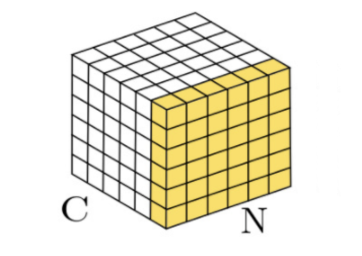
Figure above, visualizes the concept behind Batch Normalization, which reveals that normalization is completed for every batch, the place all N observations are in 1 batch, and C represents the variety of Channels or options in your information. Basically, this determine reveals that batch normalization is normalizing the information per 1 function (throughout single channel) and for all N observations in 1 batch.

This is achieved by adjusting and scaling the activations throughout coaching. Batch normalization permits every layer of a community to be taught by itself somewhat extra independently of different layers. Let’s see the way it works in additional element.

Step 1: Mini-batch Mean & Variance:

Compute the imply of the activations for a mini-batch utilizing the next equation:

$$
mu_B = frac{1}{m} sum_{i=1}^{m} x_i
$$

In this equation,

• μ_beta​ is the imply of the mini-batch
• m is the variety of coaching examples in mini-batch, and
• xi​ is the activation of the present layer earlier than batch normalization.

Now, you may must compute the variance of the activations for a mini-batch. You can do this utilizing the next equation:

$$
sigma_B^2 = frac{1}{m} sum_{i=1}^{m} (x_i – mu_B)^2
$$

Step 2: Normalize activations of the mini-batch

Then the normalization occurs:

$$
hat{x}_i = frac{x_i – mu_B}{sqrt{sigma_B^2 + epsilon}}
$$

In this equation,

• x^i​ is the normalized activation
• ϵ is a small fixed added for numerical stability (to keep away from division by zero).

Step 3: Apply the learnable parameters for scale and shift

$$
y_i = gamma hat{x}_i + beta
$$

While the first objective of batch normalization is to stabilize and speed up deep neural networks’ coaching course of by lowering inside covariate shift, it additionally has a regularization impact which is the way in which of lowering overfitting.

By including some stage of noise to the activations (for the reason that imply and variance are estimated from the information), it will probably make the mannequin much less delicate to the precise weights of neurons, which has the same impact to dropout as it will probably stop overfitting.

Batch normalization might be notably helpful in deep neural networks, the place it will probably allow the usage of larger studying charges, make the community much less delicate to the initialization, and may scale back want for different regularization methods akin to dropout.

In follow, batch normalization is utilized earlier than the activation perform of a layer, and it requires sustaining a working common of the imply and variance for use throughout inference for the normalization course of.

Chapter 6: Vanishing Gradient Problem

As the gradient of the loss is propagated backward via time and layers, it will probably shrink in direction of 0 (changing into very small). This results in very small updates to the weights.

This makes it arduous for neural community to be taught long-range dependencies, leading to doubtlessly no updates within the earlier layers of the community within the parameters because the gradients vanishes (turn into very small, near zero).

So, when gradients vanish, early layers within the community practice very slowly or in no way, resulting in suboptimal efficiency.

Use acceptable activation capabilities

One manner of fixing the vanishing gradient downside is by utilizing an acceptable activation perform that does not undergo from saturation.

Saturation occurs when, for the enter worth x that may be a giant optimistic quantity or a small unfavourable quantity, the gradient of the perform is near 0 because the perform worth is within the neighbourhood of the static excessive values of it. This slows down the parameter replace. This phenomenon is known as the saturation downside.

The ReLU (Rectified Linear Unit) and Leaky ReLU activation capabilities don’t saturate within the optimistic course, not like the Sigmoid or tanh capabilities. This might help mitigate the vanishing gradient downside.

Leaky ReLU might help additional by permitting a small, non-zero gradient when the unit shouldn’t be lively. This is essential for circumstances when the unfavourable inputs must also be considering and doubtlessly getting unfavourable worth within the output is appropriate.

You can discover extra particulars on this activation perform within the part on Activation Functions in Chapter 2.

Use Xavier or He Initialization

Initializing weights rigorously is essential. A very good initialization as such the Xavier initialization might help to stop gradients from changing into too small early in coaching.

Xavier initialization, which is also referred to as Glorot initialization, is a an initialization method for the load parameters in a neural community. It is designed to unravel the issue of vanishing or exploding gradients in deep neural networks when Sigmoid and tanh activation capabilities are getting used.

It is known as after Xavier Glorot who formulated this technique based mostly on the understanding of the circulation of variances via a neural community to take care of the gradients at an affordable scale and forestall them from changing into too small to fade or too giant to blow up.

Here’s the primary thought behind Xavier Initialization:

• For a given layer, the weights are initialized randomly from a distribution with imply 0 and a selected variance (can be 1 like in Gaussian distribution) that is determined by the variety of enter neurons and the variety of output neurons.
• The objective of Xavier Initialization is to have the variance of the outputs of every layer to be equal to the variance of its inputs, and the gradients to have equal variance earlier than and after going via a layer within the backward propagation.

If it is a Uniform Distribution, the weights are often initialized with values drawn from this calculation:

$$
W sim textual content{Uniform}left(-sqrt{frac{6}{n_{textual content{in}} + n_{textual content{out}}}}, sqrt{frac{6}{n_{textual content{in}} + n_{textual content{out}}}}proper)
$$
$$
textual content{Var}(W) = frac{2}{sqrt{n_{textual content{in}} + n_{textual content{out}}}}
$$

This variance for initializing the weights in Neural Network is usually set to this worth above referred by Var(W) – as in Variance of Weights matrix W, the place:

• n_in​ is the variety of neurons feeding into the layer
• n_out​ is the variety of neurons the outcomes are fed into (that’s, variety of neurons within the subsequent layer)

If a Normal Distribution is used as a substitute, then the weights are drawn from this one:

$$
W sim textual content{Normal}left(0, sqrt{frac{2}{n_{textual content{in}} + n_{textual content{out}}}}proper)
$$
$$
textual content{Var}(W) = frac{2}{sqrt{n_{textual content{in}} + n_{textual content{out}}}}
$$

Perform Batch Normalization

Performing batch normalization on the enter layer might help preserve a imply output near 0 and a typical deviation near 1 like Standard Normal Distribution. This prevents the gradients from changing into too small.

By Normalizing the activations, you immediately stabilize the community however not directly additionally management the weights change of your community. This implies that the gradients keep extra fixed, and as an oblique end result, BatchNorm gradients won’t vanish nor explode.

Add Residual Connections (particularly to RNNs or LSTMs)

Residual connections provide modern optimization outcomes for coaching deep neural networks, particularly on the subject of combating the vanishing gradients downside.

This is especially an issue when coping with recurrent neural networks (RNNs) or Long Short-Term Memory networks (LSTMs), that are inherently deep as a result of their sequential nature. Incorporating residual connections into RNNs or LSTMs can considerably enhance their studying capabilities.

RNNs and LSTMs are specialised for dealing with sequences of information, making them perfect for duties like language modeling and time sequence evaluation. But because the sequence size will increase, these networks are likely to undergo from the vanishing gradient downside.

To tackle this, typically residual connections are used for RNNs and LSTMs. By including a shortcut that bypasses a number of layers, a residual connection permits the gradient to circulation via the community extra immediately. In the context of RNNs and LSTMs. This means connecting the output of 1 timestep not solely to the following timestep but in addition to 1 or a number of subsequent timesteps.

How to Implement Residual Connections in RNNs and LSTMs

The implementation technique for residual connections in RNNs and LSTMs is easy. For every timestep, we modify the community such that the output shouldn’t be solely a perform of the present enter and the earlier hidden state, however in order that it additionally consists of the enter immediately.

This course of might be described as follows the place we add x to output F(x). You can even see the direct path for the gradient to circulation into the community and the mathematical derivation based mostly on this technique of including enter to output:

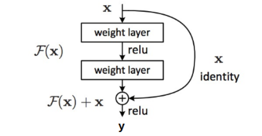
$$
y = x + F(x)
$$
$$
frac{partial E}{partial x} = frac{partial E}{partial y} cdot frac{partial y}{partial x}
$$
$$
frac{partial E}{partial x} = frac{partial E}{partial y} cdot (1 + F'(x))
$$
$$
frac{partial E}{partial x} = frac{partial E}{partial y} cdot F'(x)
$$

Here you may see the arithmetic behind Residual Connections and the way the gradient will get the short-cut. When we add x on F(x) to get y, as a substitute of simply y=F(x), you may see that after we take the spinoff of some perform E (to illustrate our loss perform) with regard to x. Then we use the chain rule from differential arithmetic.

After these transformations, you may see that we find yourself having sum of two values:

• Gradient of loss perform with regard to y
• Gradient of loss perform with regard to y multiplied by partial spinoff of F(x) with regard to x

So, you may see right here, that in case when residual connection is completed, and we add further x the plain y = F(x) , then this find yourself including further Gradient of loss perform with regard to y with out some other multiplication issue to be added to the ultimate gradient.

For intuitive and detailed clarification, try this tutorial-interview reply on Residual Connections.

Direct Gradient Flow: By offering a shortcut for the gradient to circulation, it’s much less more likely to vanish as it’s propagated again via time. This ensures that even the earliest layers within the sequence might be successfully educated.

Learning Identity Mappings: If the optimum perform for a timestep is to repeat its enter to the output, the community can be taught this identification mapping extra simply with residual connections. The community can thus concentrate on fine-tuning deviations from the identification slightly than studying it from scratch.

Facilitating Deeper Architectures: With the mixing of residual connections, it turns into possible to assemble deeper RNNs or LSTMs. This depth permits the community to be taught extra complicated patterns and relationships inside the information.

Chapter 7: Combatting Exploding Gradients

Exploding gradients is the other downside of Vansihing Gradients. Exploding Gradients happen when within the coaching of deep studying fashions, notably these involving neural networks throughout the backpropagation section, the gradients turn into too giant they usually mainly explode.

But in deep networks with many layers, these gradients can accumulate and develop exponentially giant via every layer. This exponential enhance is as a result of repetitive multiplication of gradients via the community’s depth, particularly when the gradients are too giant of their magnitude.

This hinders the educational course of and makes the neural community much less efficient in studying the essential info within the layers.

Let’s take a look at how we will resolve this downside.

Gradient Clipping

One manner of fixing the exploding gradients downside is by utilizing Gradient Clipping. Gradient clipping is a sensible method that’s used to stop gradients from exploding throughout the coaching of neural networks.

When the computed gradients are too giant, gradient clipping scales them again to a predefined threshold. This ensures steady and constant updates to the mannequin’s parameters.

This course of entails:

• Step 1: Calculating gradient (g): Obtain the gradient of the loss perform with respect to the mannequin’s parameters.
• Step 2: Scaling gradient: If the norm of this gradient ∥g∥ is bigger than a specified threshold c, we scale down gradient g to have the norm c, sustaining its course. This is completed by setting g to  c⋅g/∥g∥
• Step 3: Update parameters: We use the clipped gradient for a managed and extra reasonable replace.

Gradient clipping ensures that the mannequin’s studying course of doesn’t derail as a result of these giant updates because of exploding gradients, which might occur within the presence of steep slopes within the loss panorama when optimization ought to occur after backpropagation.

By conserving these updates of the load and bias parameters inside a ‘secure’ dimension, this technique helps in navigating the loss panorama extra easily, contributing to raised coaching convergence. The threshold cc is a hyperparameter that requires tuning to steadiness between enough studying velocity and stability.

Chapter 8: Sequence Modeling with RNNs & LSTMs

In this chapter, you may study probably the most in style kind of Neural Network fashions, Recurrent Neural Networks (RNNs).

Sequence modeling is a cornerstone of deep studying for sequential information akin to time-series, speech, and textual content. We’ll look into the mechanics of RNNs, their inherent limits, and the evolution of superior architectures akin to Long Short-Term Memory (LSTM).

Recurrent Neural Networks (RNN) Architecture

RNNs stand out for his or her distinctive means to kind a directed graph alongside a sequence, permitting them to exhibit temporal dynamic habits. Unlike feedforward, in regular neural networks, RNNs can use their inside state (reminiscence) to course of sequences of inputs.

At the core of RNN is the idea of a cell, which is the repeating unit that types the bottom of the RNN’s means to take care of a reminiscence throughout enter sequences (the tine and sequence aspect). At excessive stage, RNN might be visualized as follows:

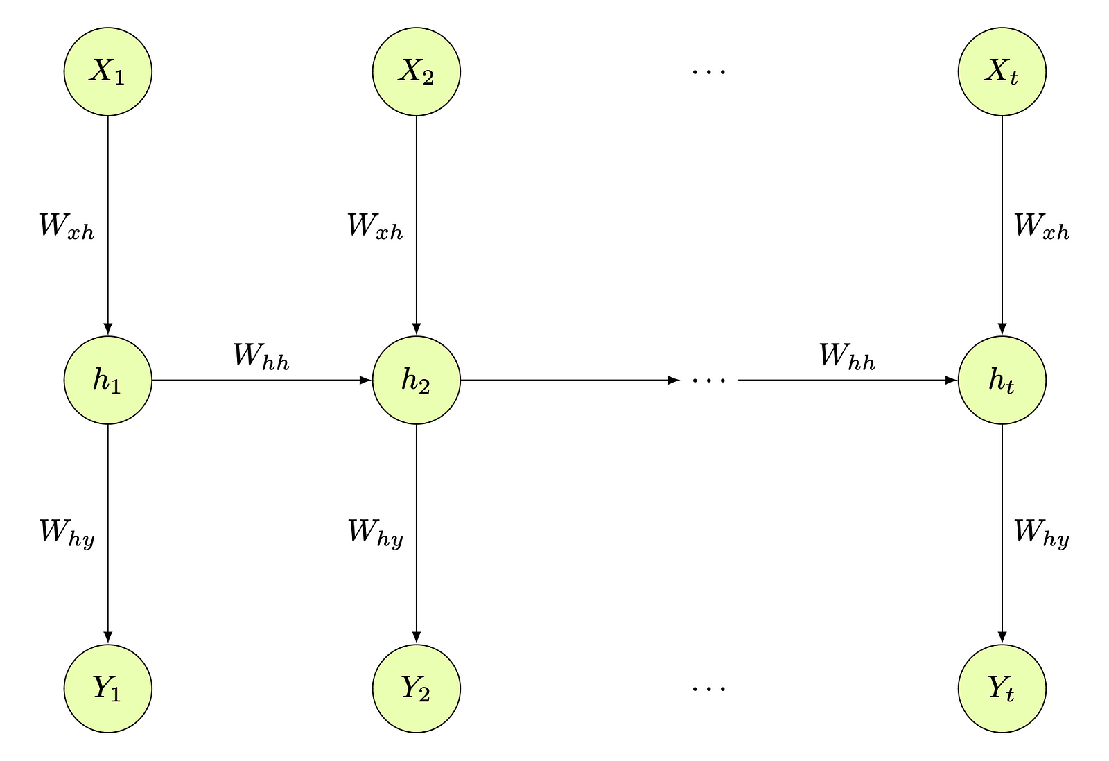
This visualization makes understanding this extra complicated structure simpler. As you may see within the picture, the hidden layer used on a selected commentary of an information set shouldn’t be solely used to generate an output for that commentary (output y utilizing h_t), however it is usually used to coach the hidden layer of the following commentary (h_t is used with x_(t+1) to get the h_(t+1)).

Unlike fundamental Neural Networks which have a single enter, a number of impartial hidden layers, after which single output Y, RNNs have a unique structure.

Besides having a unique construction for enter and output (that’s, a number of inputs and outputs), crucial factor to note right here is that in an RNN’s hidden layers, the hidden states are interconnected.

This “dependent” property of 1 commentary serving to to foretell the following commentary is why recurrent neural networks are so helpful on the subject of issues with time or sequence components (akin to time sequence evaluation issues or next-word prediction issues kind NLP).

Recurrent Neural Network Pseudocode

For the beginning, let’s search for occasion on the first time step. The hidden state at time step 1 is calculated as follows:

$$
h_1 = f(W_{xh} cdot X_1 + W_{hh} cdot h_0 + b_h)
$$

the place:

• f is an activation perform (like ReLU or Tanh)
• W_xh is the input-to-hidden weight matrix
• W_hh is the hidden-to-hidden weight matrix
• h_0 is the preliminary hidden state (earlier)
• b_h is the hidden layer bias

W_hh is sometimes called the recurrent weight matrix. This is the matrix that defines how a lot every of these earlier hidden states will contribute to the computation of the current hidden state.

Then the output on this first time-step is the next:

$$
Y_1 = W_{hy} cdot h_1 + b_y
$$

the place:

• W_hy​ is the load matrix from hidden to output layer
• b_y​ is the bias for the output layer

The RNN algorithm for all time-steps 1 until T might be described with the next pseudocode:

Algorithm 1 Recurrent Neural Network Time Steps
1: for every time step t = 1 to T do
2:     Input: Xt
3:     Initialize: h0 to a vector of zeros
4:     Parameters:
5:         Wxh: Weight matrix from enter to hidden layer
6:         Whh: Recurrent weight matrix for hidden layer
7:         Why: Weight matrix from hidden to output layer
8:         bh: Bias for hidden layer
9:         by: Bias for output layer
10:     Activation perform: f (e.g., tanh, ReLU)
11:     Hidden State Update:
12:         ht = f(Wxh . Xt + Whh . ht−1 + bh)
13:     Output:
14:         Yt = Why . ht + by
15: finish for

Limitations of Recurrent Neural Networks

Now let’s talk about the constraints of RNNs and why LSTMs got here into play in addition to afterward the Transformers! Following are the constraints of the Recurrent Neural Network:

• Vanishing Gradient Problem
• Exploding Gradient Problem
• Serial Computation
• Difficulty Handling Long Sequences
• Limited Contextual Information

Since we have already mentioned the Vanishing and Exploding Gradient issues and methods to resolve them, we’ll transfer on to the remaining limitations of RNN earlier than discussing variations of RNNs that addresses these challenges.

But first, simply to notice: particularly in case of RNNs, Vanishing Gradient can lead to the early layers of the community studying very slowly, if in any respect, which makes RNNs poorly suited to studying long-range dependencies inside a sequence. And within the case ofExploding Gradients, they will result in giant updates to community parameters and consequently to an unstable Recurrent Neural Network.

Serial Computation Limitation

The sequential nature of RNNs doesn’t enable for parallelization throughout coaching as a result of the computation of the following step is determined by the earlier step. This can lead to a lot slower coaching processes in comparison with neural networks that do enable full parallelization.

Difficulty Handling Long Sequences

RNNs can have problem when coping with lengthy sequences as a result of info from early within the sequence might be misplaced by the point it reaches the tip in case Vanishing Gradient is a matter.

Limited Contextual Information Limitation

This is without doubt one of the most essential limitations that RNN has that motivated the invention of Transformers. Standard RNNs do not need a mechanism to selectively bear in mind or overlook info, which could be a limitation when processing sequences the place solely sure components are related for the prediction.

Long Short-Term Memory (LSTM) Architecture

Long Short-Term Memory Networks or LSTMs are a particular form of RNN designed to mitigate many of the limitations of conventional RNNs. They incorporate mechanisms that we name Cells that enable the community to control the knowledge that flows via it.

These gates are:

• Forget Gate: Gate that determines what info needs to be discarded from the cell state
• Input Gate: Gate that updates the cell state with new info
• Output Gate: Gate that determines what subsequent hidden state needs to be

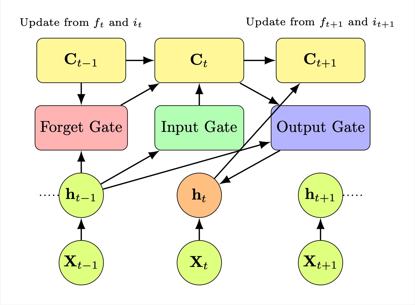
This diagram represents the structure of an LSTM (Long Short-Term Memory) community, visualizing the circulation of information via its elements at totally different time steps, let’s dive deeper into every of this sates and the method behind them:

Cell States: At the highest row, we now have rectangles in yellow labeled C_(t−1), C_(t)​, … C_(t+1)​. These signify the cell states of LSTM at consecutive time steps.

These cell states are a key element of the LSTM as they carry related info all through processing of the sequence. They maintain the knowledge of what info to make use of, what to overlook and what to output.

Arrows point out the circulation and transformations of the cell state from one time step to the following one.

Gates: In the center you may see the three gates, colored blocks representing the LSTM’s gates:

• Forget Gate (Pink): Determines which components of cell state C_(t−1)​ must be forgotten and which have to be remembered, to supply the next cell state C_(t)​.
• Input Gate (Green): Decides which values can be up to date within the cell state based mostly on the enter on the present time step.
• Output Gate (Purple): Determines what a part of the cell state can be used to generate the output hidden state h_t​.

These 3 gates management the circulation of knowledge and their quantity, with traces connecting the earlier hidden state h_(t−1) ​and the cell state to every of those gates, illustrating how every of them contribute to the present state.

Difference between Cell and Gates: Note, that cells and gates are totally different ideas, the place as you may see from the diagram cell is at larger leven than the gates, and for every time step there’s single cell state however 3 gates. Cell state is mainly utilizing 3 gates to control the circulation of knowledge. It’s like perform that makes use of 3 enter values to generate output to place it merely.

Common to the RNN unique structure, the hidden state at every time step is influenced by the earlier hidden state and present enter, and in addition the inner gates’ operations widespread for LSTMs.

These gates inside LSTM enable it to be taught which info to maintain or discard over time, making it potential to seize long-term dependencies within the information.

How LSTMs tackle RNN limitations

• Solving Vanishing and Exploding Gradients: LSTMs are designed to have a extra fixed weight adjustments which implies that the gradients are extra fixed. This permits them to be taught over many time steps, thereby fixing the vanishing/exploding gradients via their gating mechanism and by sustaining a separate cell state.
• Long-range Dependencies: By studying what to retailer in and what to delete/overlook from the cell state, LSTMs can preserve long-range dependencies or relationships within the information. This makes them more practical for duties involving lengthy sequences akin to these in language fashions.
• Selective Memory: LSTMs can be taught to maintain solely related info to make predictions by utilizing the, overlook gate. Forgetting non-relevant information, which makes them higher at modeling complicated sequences the place the relevance of the knowledge varies with time helps to do precisely this.

Limitations of LSTMs

While LSTMs signify a big enchancment over the unique RNNs, they nonetheless have some main disadvantages, akin to being extra computationally intensive as a result of their complicated structure. LSTM’s have the next variety of parameters, which might result in longer coaching instances and require extra information to generalize successfully.

Also, much like RNNs, LSTMs additionally course of information sequentially, which suggests they can’t be totally parallelized.

So, parallelization and longer coaching time as a result of larger variety of parameters stay two main disadvantages for RNNs and LSTMs.

Chapter 9: Deep Learning Interview Preparation

As we attain the end result of this complete handbook, it’s time to concentrate on translating your newfound data into real-world success.

Whether you are aiming for entering into AI business or eyeing a coveted place for AI Researcher or AI Engineer at FAANG firms, the ultimate hurdle is commonly probably the most difficult but rewarding: the job interview.

You might want to know particulars and be capable of reply tough questions that transcend the floor stage concept info.

You’ll must learn about:

• Convolutional Neural Networks (pooling, padding, kernels)
• Recurrent Neural Networks (RNN), LSTMs, GRUs
• Batch/Layer Normalization
• Generative Adverserial Networks (GANs)
• AutoEncoders (Encoder-Decoder Architectures)
• Variational AutoEncoders (KL Divergence, ELBO)
• Embeddings
• Multi-Head Attention Mechanism
• Transformers

And these are simply few subjects which you can anticipate on your extra superior/FAANG interviews. Check out the complete checklist of 100 Questions from this curriculum of right here.

Understanding the significance of this vital step, I’m excited to introduce my specifically designed Deep Learning Interview Course sponsored by LunarTech that is obtainable on LunarTech.ai and Udemy. This course is meticulously tailor-made to make sure you aren’t simply interview-ready however poised to excel within the extremely aggressive AI job market.

Here’s what the course covers:

1. Part 1 – The Essentials (Free 4-Hour Course): I consider in empowering each Data Science AI fanatic. So I’m providing the primary a part of my interview course completely free. This part consists of first set of fifty interview questions that cowl the breadth of deep studying fundamentals.
2. Complete Course – [Full Deep Learning Interview Prep Course – 100 Q&A 7.5 hours ]: For those that are decided to depart no stone unturned, our full course on LunarTech.ai is the final word preparation instrument for simple but in addition complicated Deep Learning interviews. Expanding to 100 in-depth interview questions, this complete course delves into the nuances of deep studying, guaranteeing that you just stand out in even probably the most demanding interviews, together with firms like FAANG.

It’s your alternative to transcend being a candidate – to changing into a standout within the subject of AI.

About the Author

I’m Tatev Aslanyan, Senior Machine Learning and AI Researcher. I’ve had the privilege of working in Data Science throughout quite a few international locations, together with the US, UK, Canada, and the Netherlands. I’m Co-founder of LunarTech the place make Data Science and AI extra accessible to everybody!

With an MSc and BSc in Econometrics beneath my belt, my journey in Machine and AI has been nothing wanting unbelievable. Drawing from my technical research throughout my Bachelors & Masters, together with over 5 years of hands-on expertise within the Data Science, Machine Learning and AI business.

Connect with Me and LunarTech

If you need to begin a profession in Data Science or AI, obtain my free Data Science and AI Handbook or Fundamentals to Machine Learning Handbook

Best needs in all of your future endeavors!