
Binary classification is a elementary job in machine studying, the place the objective is to categorize knowledge into certainly one of two courses or classes.
Binary classification is utilized in a variety of purposes, equivalent to spam e mail detection, medical analysis, sentiment evaluation, fraud detection, and plenty of extra.
In this text, we’ll discover binary classification utilizing TensorFlow, one of the vital in style deep studying libraries.
Before entering into the Binary Classification, let’s focus on slightly about classification downside in Machine Learning.
What is Classification downside?
A Classification downside is a kind of machine studying or statistical downside wherein the objective is to assign a class or label to a set of enter knowledge based mostly on their traits or options. The goal is to be taught a mapping between enter knowledge and predefined courses or classes, after which use this mapping to foretell the category labels of latest, unseen knowledge factors.
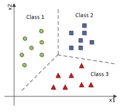
The above diagram represents a multi-classification downside wherein the information might be categorized into greater than two (three right here) kinds of courses.
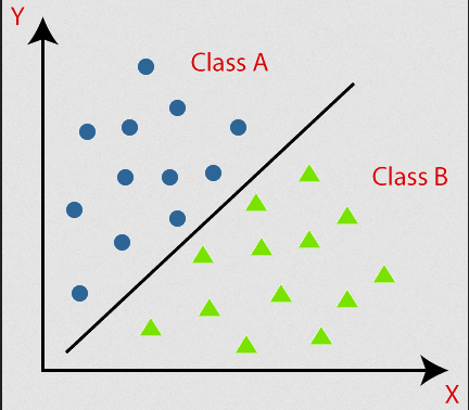
This diagram defines Binary Classification, the place knowledge is assessed into two sort of courses.
This easy idea is sufficient to perceive classification issues. Let’s discover this with a real-life instance.
Heart Attack Analytics Prediction Using Binary Classification
In this text, we are going to embark on the journey of developing a predictive mannequin for coronary heart assault evaluation using easy deep studying libraries.
The mannequin that we’ll be constructing, whereas being a comparatively easy neural community, is able to reaching an accuracy degree of roughly 80%.
Solving real-world issues by way of the lens of machine studying entails a collection of important steps:
- Data Collection and Analytics
- Data preprocessing
- Building ML Model
- Train the Model
- Prediction and Evaluation
Data Collection and Analytics
It’s price noting that for this venture, I obtained the dataset from Kaggle, a well-liked platform for knowledge science competitions and datasets.
I encourage you to take a more in-depth have a look at its contents. Understanding the dataset is essential because it lets you grasp the nuances and intricacies of the information, which may also help you make knowledgeable selections all through the machine studying pipeline.
This dataset is well-structured, and there is not any speedy want for additional evaluation. However, if you’re accumulating the dataset by yourself, you will want to carry out knowledge analytics and visualization independently to attain higher accuracy.
Let’s placed on our coding sneakers.
Here I’m utilizing Google Colab. You can use your individual machine (wherein case you will want to create a .ipynb file) or Google Colab in your account to run the pocket book. You can discover my supply code right here.
As step one, let’s import the required libraries.
import numpy as np
import matplotlib.pyplot as plt
from sklearn.model_selection import train_test_split
import sklearn
import pandas as pd
import keras
from keras.fashions import Sequential
from keras.layers import Dense
import tensorflow as tf
from sklearn.metrics import confusion_matrix,ConfusionMatrixDisplay
from sklearn.preprocessing import MinMaxScalerI’ve the dataset in my drive and I’m studying it from my drive. You can obtain the identical dataset right here.
Remember the change the trail of your file within the read_csv methodology:
df = pd.read_csv("/content material/drive/MyDrive/Datasets/coronary heart.csv")
df.head()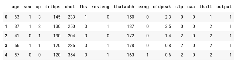
The dataset comprises 13 enter columns (age, intercourse, cp, and so forth) and one output column (output), which is able to comprise the information as both 0 or 1.
Considering the enter readings, 0 within the output represents the individual won’t get coronary heart assault, whereas the 1 represents the individual might be affected by coronary heart assault.
Let’s break up our enter and output from the above dataset to coach our mannequin:
target_column = "output"
numerical_column = df.columns.drop(target_column)
output_rows = df[target_column]
df.drop(target_column,axis=1,inplace=True)Since our goal is to foretell the probability of a coronary heart assault (0 or 1), represented by the goal column, we break up that right into a separate dataset.
Data preprocessing
Data preprocessing is a vital step within the machine studying pipeline, and binary classification is not any exception. It entails the cleansing, transformation, and group of uncooked knowledge right into a format that’s appropriate for coaching machine studying fashions.
A dataset will comprise a number of sort of information equivalent to Numerical Data, Categorical Data, Timestamp Data, and so forth.
But a lot of the Machine Learning algorithms are designed to work with numerical knowledge. They require enter knowledge to be in a numeric format for mathematical operations, optimization, and mannequin coaching.
In this dataset, all of the columns comprise numerical knowledge, so we needn’t encode the information. We can proceed with easy normalization.
Remember if in case you have any non-numerical columns in your dataset, you’ll have to transform it into numerical by performing one-hot encoding or utilizing different encoding algorithms.
There are lot of normalization methods. Here I’m utilizing Min-Max Normalization:

Don’t fear – we needn’t apply this components manually. We have some machine studying libraries to do that. Here I’m utilizing MinMaxScaler from sklearn:
scaler = MinMaxScaler()
scaler.match(df)
t_df = scaler.remodel(df)scaler.match(df) computes the imply and customary deviation (or different scaling parameters) essential to carry out the scaling operation. The match methodology basically learns these parameters from the information.
t_df = scaler.remodel(df): After becoming the scaler, we have to remodel the dataset. The transformation sometimes scales the options to have a imply of 0 and a typical deviation of 1 (standardization) or scales them to a particular vary (for instance, [0, 1] with Min-Max scaling) relying on the scaler used.
We have accomplished the preprocessing. The subsequent essential step is to separate the dataset into coaching and testing units.
To accomplish this, I’ll make the most of the train_test_split operate from scikit-learn.
X_train and X_test are the variables that maintain the impartial variables.
y_train and y_test are the variables that maintain the dependent variable, which represents the output we’re aiming to foretell.
X_train, X_test, y_train, y_test = train_test_split(t_df, output_rows, test_size=0.25, random_state=0)print('X_train:',np.form(X_train))
print('y_train:',np.form(y_train))
print('X_test:',np.form(X_test))
print('y_test:',np.form(y_test))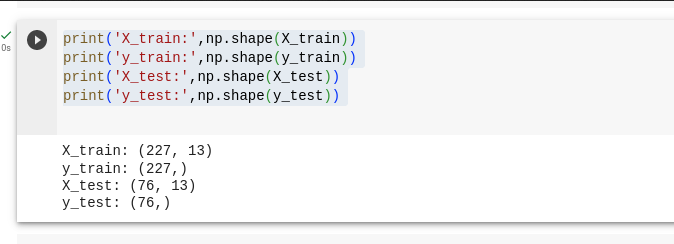
We break up the dataset by 75% and 25%, the place 75% goes for coaching our mannequin and 25% goes for testing our mannequin.
Building ML Model
A machine studying mannequin is a computational illustration of an issue or a system that’s designed to be taught patterns, relationships, and associations from knowledge. It serves as a mathematical and algorithmic framework able to making predictions, classifications, or selections based mostly on enter knowledge.
In essence, a mannequin encapsulates the information extracted from knowledge, permitting it to generalize and make knowledgeable responses to new, beforehand unseen knowledge.
Here, I’m constructing a easy sequential mannequin with one enter layer and one output layer. Being a easy mannequin, I’m not utilizing any hidden layer as it’d enhance the complexity of the idea.
Initialize Sequential Model
basic_model = Sequential()Sequential is a kind of mannequin in Keras that lets you create neural networks layer by layer in a sequential method. Each layer is added on high of the earlier one.
Input Layer
basic_model.add(Dense(models=16, activation='relu', input_shape=(13,)))Dense is a kind of layer in Keras, representing a totally linked layer. It has 16 models, which suggests it has 16 neurons.
activation='relu' specifies the Rectified Linear Unit (ReLU) activation operate, which is often utilized in enter or hidden layers of neural networks.
input_shape=(13,) signifies the form of the enter knowledge for this layer. In this case, we’re utilizing 13 enter options (columns).
Output Layer
basic_model.add(Dense(1, activation='sigmoid'))This line provides the output layer to the mannequin.
It’s a single neuron (1 unit) as a result of this seems to be a binary classification downside, the place you are predicting certainly one of two courses (0 or 1).
The activation operate used right here is 'sigmoid', which is often used for binary classification duties. It squashes the output to a spread between 0 and 1, representing the likelihood of belonging to one of many courses.
Optimizer
adam = keras.optimizers.Adam(learning_rate=0.001)This line initializes the Adam optimizer with a studying price of 0.001. The optimizer is accountable for updating the mannequin’s weights throughout coaching to reduce the outlined loss operate.
Compile Model
basic_model.compile(loss="binary_crossentropy", optimizer=adam, metrics=["accuracy"])Here, we’ll compile the mannequin.
loss="binary_crossentropy" is the loss operate used for binary classification. It measures the distinction between the expected and precise values and is minimized throughout coaching.
metrics=["accuracy"]: During coaching, we need to monitor the accuracy metric, which tells you ways nicely the mannequin is performing by way of right predictions.
Train mannequin with dataset
Hurray, we constructed the mannequin. Now it is time to prepare the mannequin with our coaching dataset.
basic_model.match(X_train, y_train, epochs=100)X_train represents the coaching knowledge, which consists of the impartial variables (options). The mannequin will be taught from these options to make predictions or classifications.
y_train are the corresponding goal labels or dependent variables for the coaching knowledge. The mannequin will use this data to be taught the patterns and relationships between the options and the goal variable.
epochs=100: The epochs parameter specifies the variety of occasions the mannequin will iterate over all the coaching dataset. Each go by way of within the dataset is known as an epoch. In this case, now we have 100 epochs, which means the mannequin will see all the coaching dataset 100 occasions throughout coaching.
loss_and_metrics = basic_model.consider(X_test, y_test)
print(loss_and_metrics)
print('Loss=",loss_and_metrics[0])
print("Accuracy = ',loss_and_metrics[1])The consider methodology is used to evaluate how nicely the educated mannequin performs on the take a look at dataset. It computes the loss (typically the identical loss operate used throughout coaching) and any specified metrics (for instance, accuracy) for the mannequin’s predictions on the take a look at knowledge.
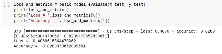
Here we acquired round 82% accuracy.
Prediction and Evaluation
predicted = basic_model.predict(X_test)The predict methodology is used to generate predictions from the mannequin based mostly on the enter knowledge (X_test on this case). The output (predicted) will comprise the mannequin’s predictions for every knowledge level within the coaching dataset.
Since I’ve solely minimal dataset I’m utilizing the take a look at dataset for prediction. However, it’s a advocate observe to separate part of dataset (say 10%) to make use of as a validation dataset.
Evaluation
Evaluating predictions in machine studying is a vital step to evaluate the efficiency of a mannequin.
One generally instrument used for evaluating classification fashions is the confusion matrix. Let’s discover what a confusion matrix is and the way it’s used for mannequin analysis:
In a binary classification downside (two courses, for instance, “constructive” and “unfavorable”), a confusion matrix sometimes seems like this:
| Predicted Negative (0) | Predicted Positive (1) | |
| Actual Negative (0) | True Negative | False Positive |
| Actual Positive (1) | False Negative | True Positive |
Here’s the code to plot the confusion matrix from the expected knowledge of our mannequin:
predicted = tf.squeeze(predicted)
predicted = np.array([1 if x >= 0.5 else 0 for x in predicted])
precise = np.array(y_test)
conf_mat = confusion_matrix(precise, predicted)
displ = ConfusionMatrixDisplay(confusion_matrix=conf_mat)
displ.plot()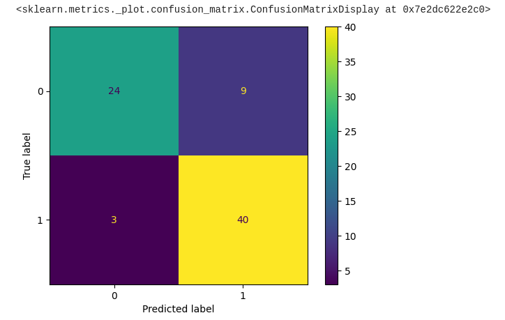
Bravo! We’ve made important progress towards acquiring the required output, with roughly 84% of the information showing to be right.
It’s price noting that we are able to additional optimize this mannequin by leveraging a bigger dataset and fine-tuning the hyper-parameters. However, for a foundational understanding, what we have completed up to now is sort of spectacular.
Given that this dataset and the corresponding machine studying fashions are at a really primary degree, it is essential to acknowledge that real-world eventualities typically contain far more complicated datasets and machine studying duties.
While this mannequin might carry out adequately for easy issues, it is probably not appropriate for tackling extra intricate challenges.
In real-world purposes, datasets may be huge and various, containing a large number of options, intricate relationships, and hidden patterns. Consequently, addressing such complexities typically calls for a extra refined method.
Here are some key elements to contemplate when working with complicated datasets.
- Complex Data Preprocessing
- Advanced Data Encoding
- Understanding Data Correlation
- Multiple Neural Network Layers
- Feature Engineering
- Regularization
If you are already aware of constructing a primary neural community, I extremely advocate delving into these ideas to excel on the earth of Machine Learning.
Conclusion
In this text, we launched into a journey into the fascinating world of machine studying, beginning with the fundamentals.
We explored the basics of binary classification—a elementary machine studying job. From understanding the issue to constructing a easy mannequin, we have gained insights into the foundational ideas that underpin this highly effective discipline.
So, whether or not you are simply beginning or already nicely alongside the trail, maintain exploring, experimenting, and pushing the boundaries of what is attainable with machine studying. I’ll see you in one other thrilling article!
If you want to be taught extra about synthetic intelligence / machine studying / deep studying, subscribe to my article by visiting my web site, which has a consolidated checklist of all my articles.